For some calculations, Google Sheets has more in-built functions compared to Excel. For Instance, to perform multiplications in Sheets, there are three different functions such as MULTIPLY, PRODUCT, and SUMPRODUCT. So, calculating the product between two or more numbers is quite easy. You wouldn’t have to enter Asterisk operator manually to multiply numbers.
Using MULTIPLY Function
If you have to multiply only two numbers or columns in Google Sheets, you could use the MULTIPLY function. For instance, to create a multiplication table in a spreadsheet. This function is just the same as using the (*) Asterisk operator to calculate the product. But, here, we will simply use the numbers or cell references in the formula.
I especially recommend you use the MULTIPLY function as you can use Sheet’s auto-fill to calculate the remaining numbers.
Syntax: MULTIPLY(factor1, factor2)MULTIPLY function takes up only two arguments which are the first multiplicand and second multiplicand. Note that this function does not accept more than two values or arguments in the formula. By chance, if you enter an extra third value, you’ll get a #N/A error in the cell.
Now, let’s take a look at the example of using MULTIPLY functions.
Example 1: Multiply Numbers
Let’s say you need to find out the product of 15 and 18. For this, you can enter the formula as
=MULTIPLY(15, 18)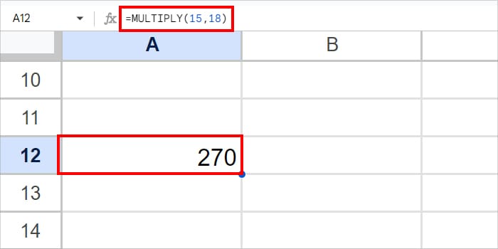
It’ll return 270.
Example 2: Multiply Relative Cells
If you have numbers in two columns to multiply, you could use a cell reference in the MULTIPLY function instead. This way, you could easily calculate the rest of the numbers with the Smart-fill feature.
Below, we have provided an example of multiplying the relative cells. Here, we will multiply each cell of Column A with Column B. For this, we entered the formula mentioned in the box.
=MULTIPLY(A2, B2)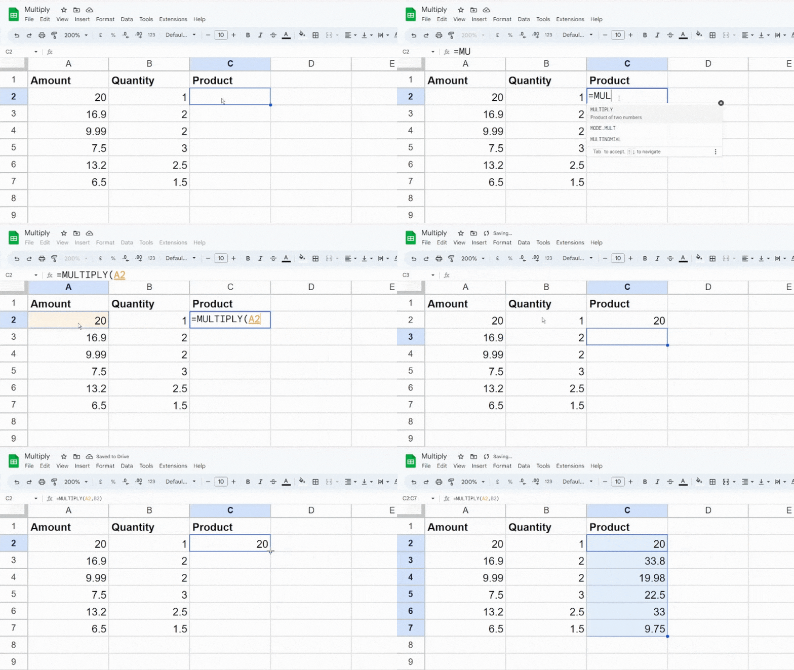
Now, we will apply the same formula to fill in the rest of the data. For this, select the formula cell and hover over the bottom-right corner of cell C1. When the Plus cursor appears, click and drag down the remaining cells.
Example 3: Multiply Absolute Cell
Sometimes, you may wish to multiply all the values of a column with just one number. For Instance, multiply the entire Column A by the number 7 in cell B2.
For this, we will lock the B2 cell in the formula to specify it as an absolute cell reference. This is because we want all the values of Column A to refer to only cell B2 for multiplication. To convert it to absolute cell reference, we will add a dollar sign in the B2 cell like this $B$2.
When you do not lock cells, the relative cell reference changes while copying down the formula. For example, cell A2 will multiply cell B2, A3 will B3, and so on. Since the remaining cell of column B is empty, it’ll only result in 0 output.
Now, to calculate the product, we will enter the formula as
=MULTIPLY(A2, $B$2)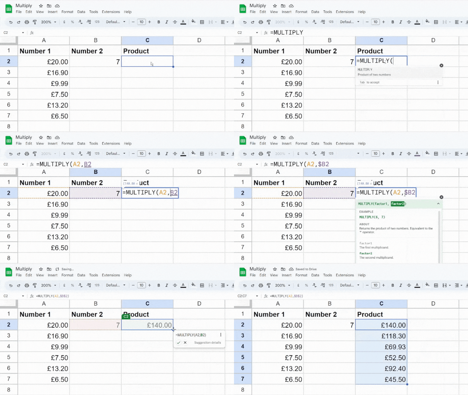
After you get the result, extend the smart-fill handle to automatically fill the other cells.
Example 4: Multiply Percentage
The MULTIPLY function also comes in handy to calculate the product of a number and percentage.
In the given data, I want to multiply all Column A with the percentage value of Column B. So, I will use the same formula as I did earlier in the Relative cell reference. Then, use Ctrl + Enter for auto-fill.
=MULTIPLY(A2, B2)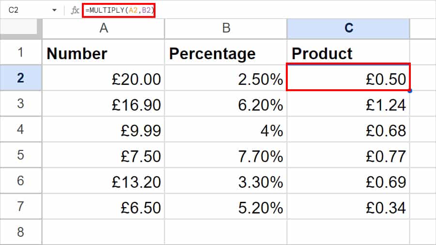
Alternatively, if you have a single percentage number to multiply, you can enter the formula as
=MULTIPLY(A11, $B$11)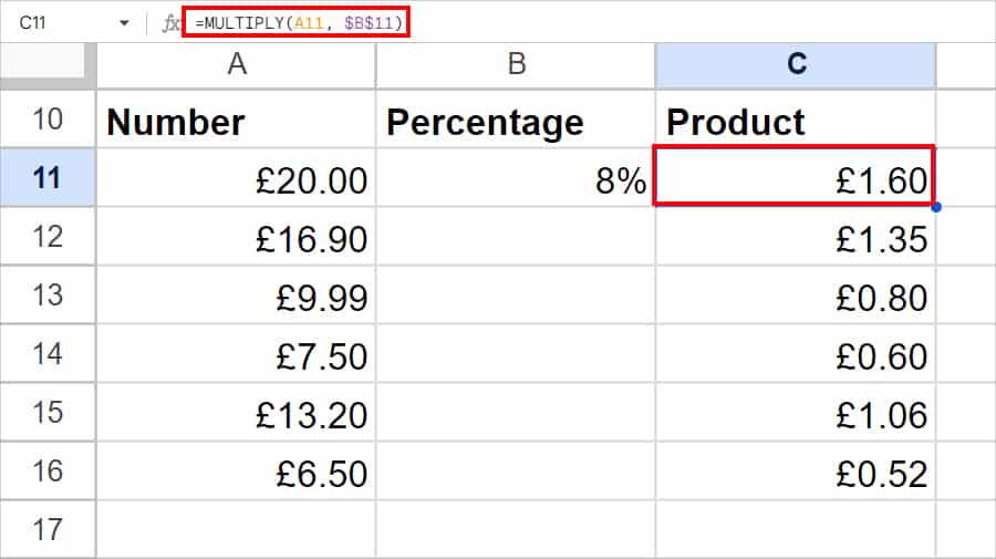
Using PRODUCT Function
There can be situations where you need to multiply an array of cell ranges in Google Sheets. In that case, you could opt for the PRODUCT function as it returns the product of a series of numbers.
Syntax: PRODUCT(factor 1, [factor2,...])The PRODUCT function takes factor 1, factor 2, factor 3, and so on up to 30 arguments. There are two ways you can use the PRODUCT function. Check out the examples.
Example 1: Multiply Several Cell Ranges
Let’s assume you need to multiply cell ranges from A2 through D2. For this, we will enter the formula as
=PRODUCT(A2:D2)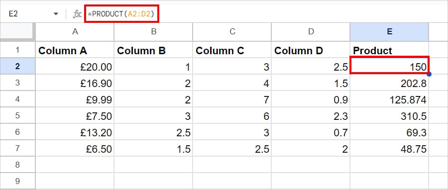
Use the Ctrl + Enter keys to fill in the remaining cells.
Example 2: Product of Cell Ranges and a Different Number
Another case of using the PRODUCT function is to multiply the ranges by a different number. Here, we will use two factor arguments in the PRODUCT function.
For example, you could multiply cell A2:D2 and again multiply the outcome by a different number. To do so, we entered the formula as
=PRODUCT(A2:D2, 2)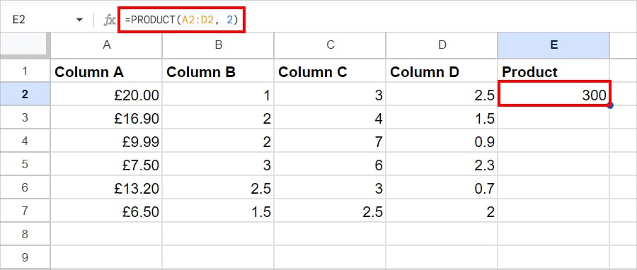
In the formula, we have passed down the value of cell A2 through D2 as factor 1 and the number 2 as a second factor. So, the formula will calculate the product of 150 and 2. Then, return 300 as a result.
Using SUMPRODUCT Function
Suppose, you need to perform both multiplication and additions in Sheet. In most cases, you would have to do this while calculating the weighted average, product bills, etc. During that time, you could opt for Sheet’s SUMPRODUCT function instead of using the SUM and PRODUCT functions differently.
Sheet’s SUMPRODUCT function multiples numbers and returns their SUM. While using this function, the first array and second array should be of same size.
Syntax: SUMPRODUCT(array1, [array2,....])In this example, we have Exams in Column A, Exam Scores in Column B, and Weighted Averages in Column C. To calculate this, we used the formula as
=SUMPRODUCT(B2:B4, C2:C4)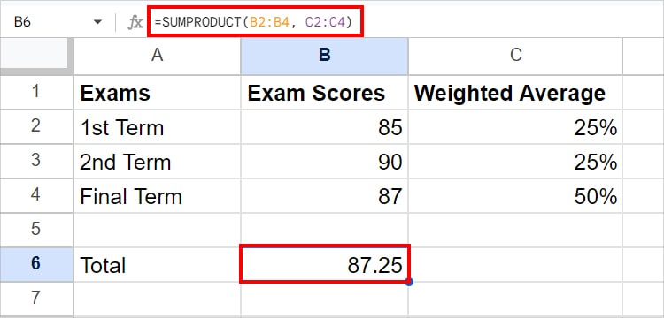
In the formula, the SUMPRODUCT function will multiply (B2 * C2) + (B3 * C3), and so on. Then, as a result, return 87.25 output.