How to Make a Gantt Chart in Excel

Need to track your project progress? 

Gantt Charts, started in the 1910s by Henry Gantt to present a project schedule with bar graphs, is now extremely popular among project managers. Over the years, it surely has advanced and comprises more elements that give a bird’s eye view of the project.

So, whether it’s your university or business project, you can use Gantt Charts to create a timeline and keep track of the task completion, progress, milestones, etc. all in one view.

Since Microsoft Excel has in-built Gantt Chart templates for 365 versions, creating them isn’t much of a big deal. But, if you use the older Excel versions, we’ve got you covered with a step-by-step guide from the most simple to advanced Gantt Chart. 

Gantt Chart for Microsoft 365 Users

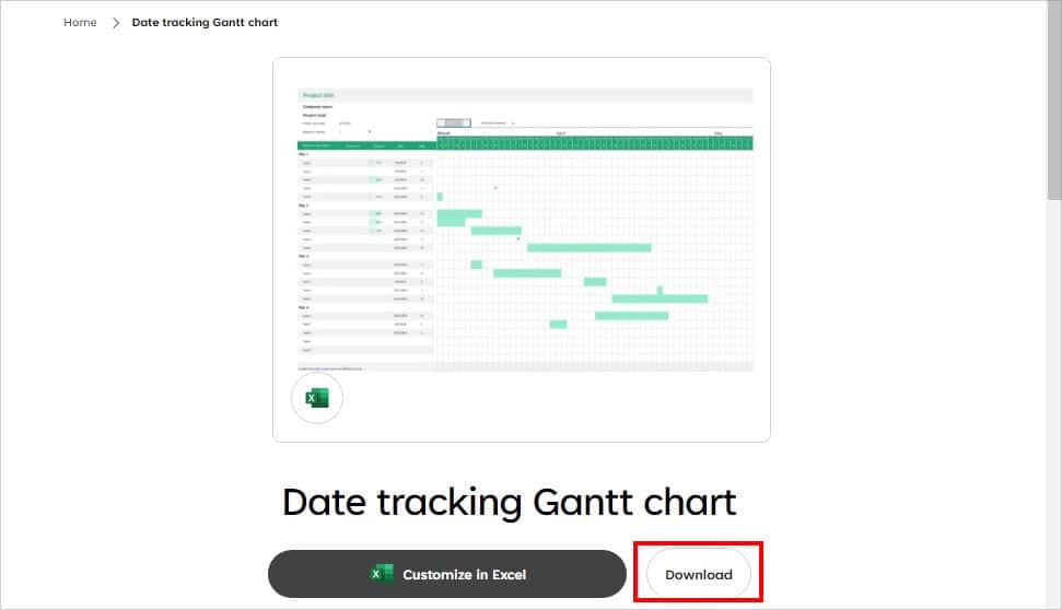
If you have a Microsoft 365 subscription, Gantt Chart templates are readily available for you. You could just download any one and customize the Chart.

1. Look for the Gantt Chart in Excel online. 
2. Choose and open the Gantt Chart template you like. Then, click on the Download.
   
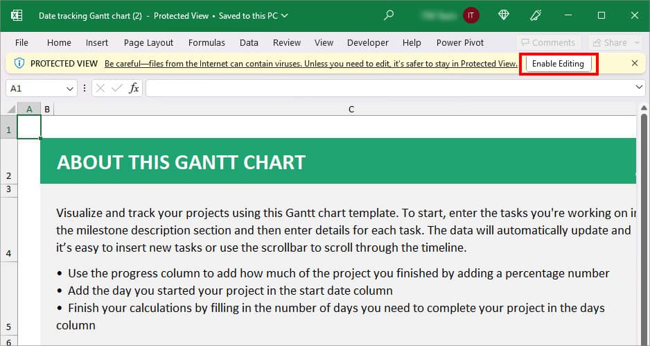
3. Open the Downloaded template in your Excel. You need to hit the Enable Editing button to make changes.
   
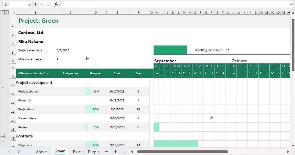
4. Now, on the About sheet, read the instructions and follow them to customize the charts.
5. You can head to another Sheet and edit the Gantt Chart. Once you’re done save the File.
   

Gantt Chart Using Charts (Older Excel Version)

Unfortunately, the built-in Gantt Chart template is limited to only the 365 users. So, if you have older Excel versions, you need to create the Gantt chart manually from square one. 

This method is for users who need to prepare a very simple Gantt Chart. For instance, Students can use this approach to make a Gantt Chart for their Thesis or Research projects. Or, a small business owner to monitor certain project progress that does not require advanced tracking.

Step 1: Prepare Data Source

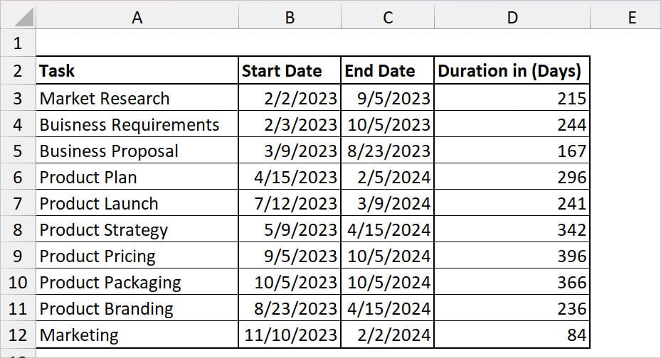
Firstly, in order to create a Gantt Chart in Excel, you need to prepare your data source. For a very basic Gantt Chart, you would need a Task, Start Date, End Date, and Duration. 

To find out the duration, you can simply subtract the End Date from the Start Date. You’ll have the number of days. However, if you have a huge gap of months, you could calculate the months between the dates. 

As an example, this is my data source to plot the Gantt Chart. I have a Product Development Project with Tasks, Dates, and Duration in days. 

Step 2: Insert Stacked Bar

1. Firstly, select your data and enter the Ctrl + T to apply the Table. Click OK in the confirmation pop-up. 
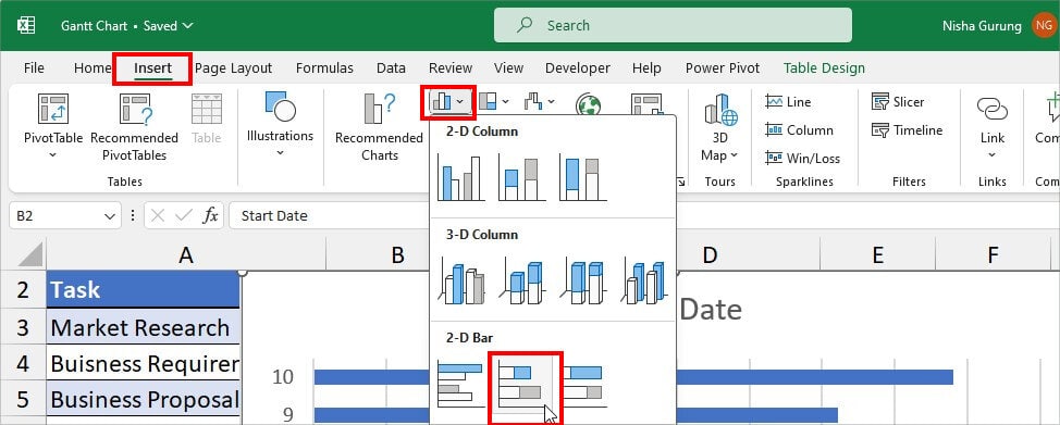
2. Now, select only the Start Date and head to the Insert Tab. 
3. On the Charts group, click on Column Chart > 2-D Stacked Column Bar.
   

Step 3: Format Data Series 

1. Right-click on the Series line and pick Select Data.
   
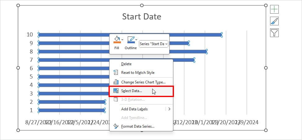
2. Below the Legend Entries (Series), click Add button.
   
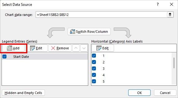
3. On Edit Series, fill in the following fields and click OK.
   
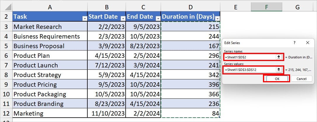
   • Series name: Select the Duration heading.
   • Series values: Select the Entire cell range for Duration. 
4. Below Horizontal (Category) Axis Labels, hit Edit.
   
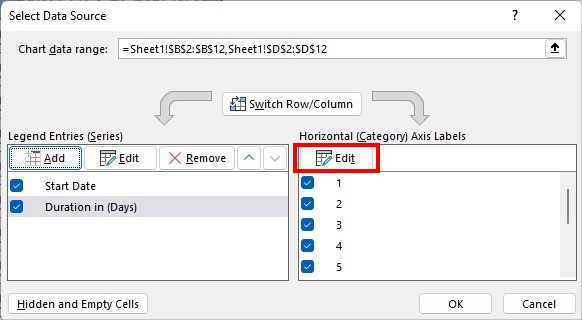
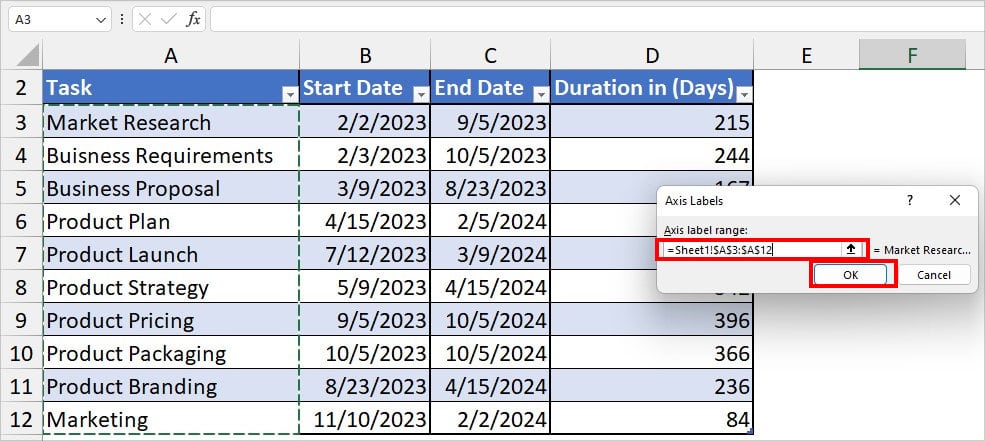
5. On Axis label range, select all ranges of Task column. Then, hit OK.
   
6. Click OK.
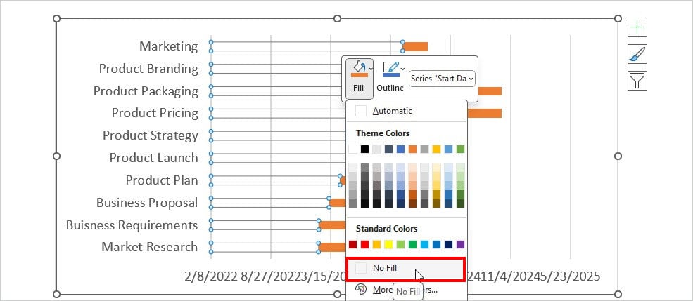
7. Right-click on the Start Date (Blue Bar) and choose No Fill.
   

Step 4: Change Axis Range

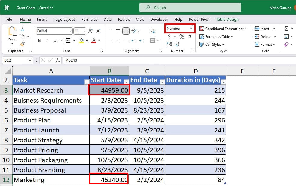
1. Firstly, change the First and Last Date from the Start Date Column into the Number format. Select the cell and click on Number format in the Home Tab.
   
2. Now, right-click on the X-Axis (Date Axis) and pick the Format Axis.
   
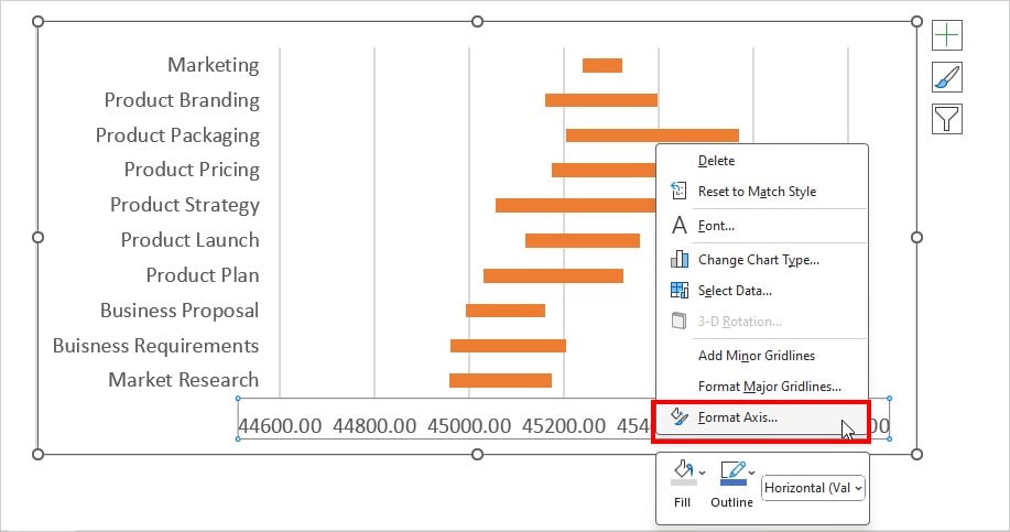
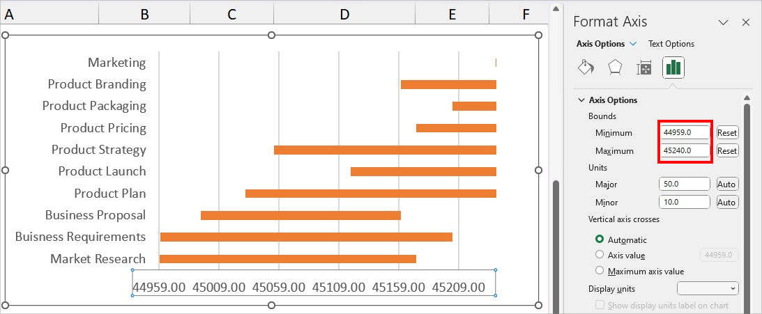
3. Under Bounds, set the Minimum number the same as the First Date. Enter the Maximum value the same as the Maximum Date.
   
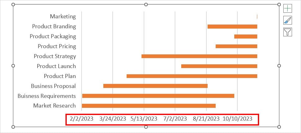
4. Once you’re done, change the Formatting back to the Date from the Home Tab. Your Dates should look clean now.
   
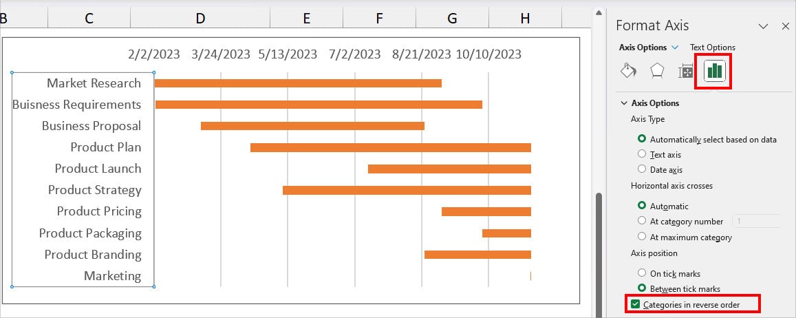
5. Double-click on the Y-Axis for the Format Axis menu. Click on Axis Options. 
6. Under, Axis Options, tick the box for Categories in reverse order.
   

Step 5: Add Chart Title

1. Select your Gantt Chart.
2. Click the + icon and tick the options for Chart Title.
   
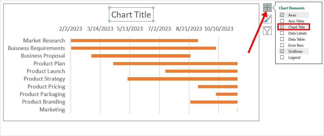
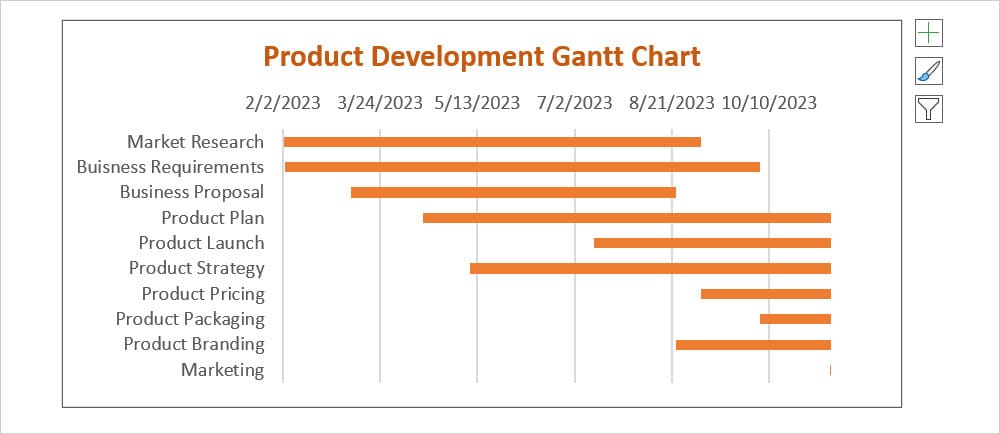
3. Rename the Chart Title. Apply the Font color and Bold text to make it stand out. Your Gantt Chart is ready!
   

Gantt Chart Using Formula (Older Excel Version)

Another way to make the Gantt Chart manually on older Excel versions is by using the formula. This method is especially effective for bigger projects and detailed monitoring. Here, we will create a more interactive and dynamic Gantt Chart. 

Step 1: Prepare Data Source

To prepare a Gantt Chart without using Excel charts, you would need a lot of information in your sheet. So, prepare your data in this order.

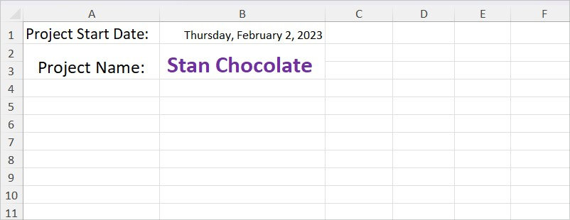
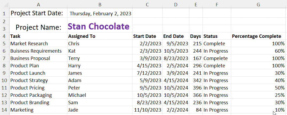
1. Firstly, enter the Project Start Date and Project Name. You can use Merge and Center for the Project Heading to highlight it.
   
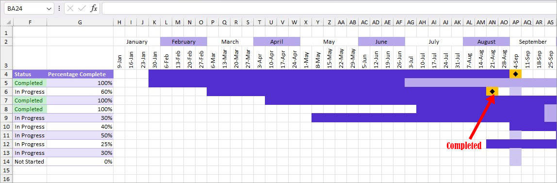
2. On the Data Table, enter your project information. Here, I have added Task, Assigned To, Start Date, End Date, Days, Status, Percentage Complete. After the data entry, I converted the cell ranges into the Table(Press Ctrl + T and click OK on the confirmation). You can change the Table Design color if you want.
   
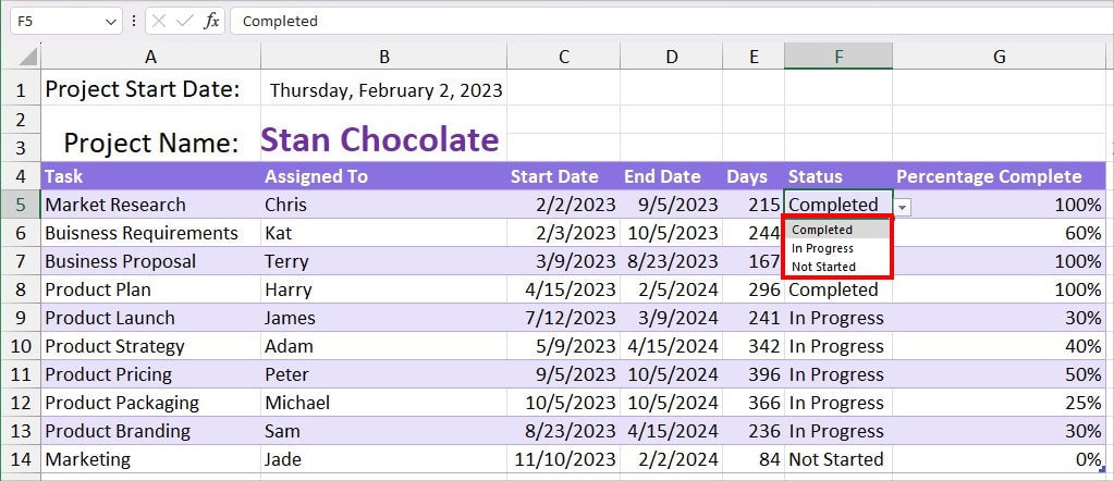
3. For the Status column, I created the Drop-down list with Completed, In Progress, and Not Started.
   
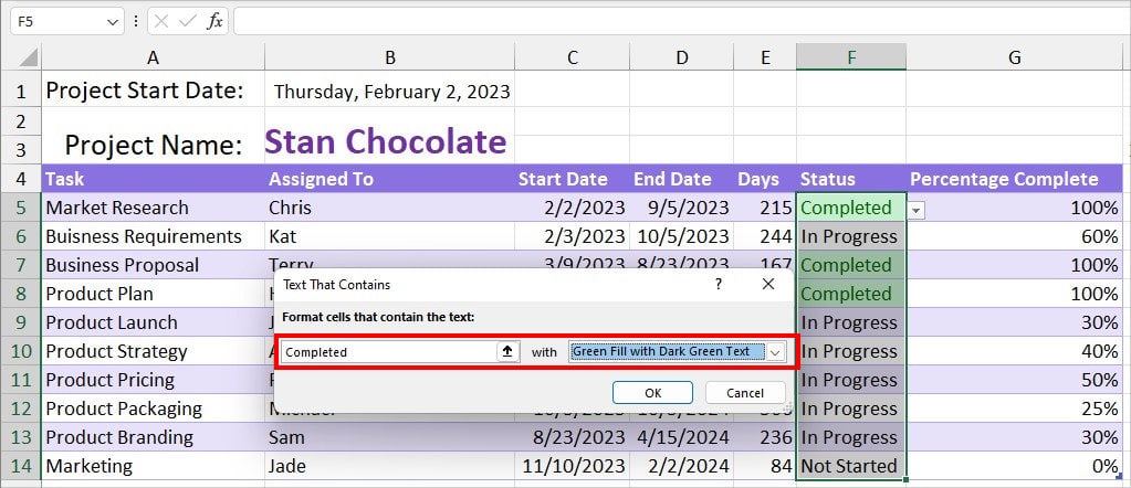
4. I used the Conditional Formatting Rule, to highlight the Completed cells with Green Colour.
   
5. Now, enter the Calendar Date for the Gantt Chart. I first entered the given formula =IF(MONTH(B1 - WEEKDAY((B1), 2) + 1) <MONTH(B1), (B1-28-DAY(B1)+7) -WEEKDAY((B1-DAY(B1)+7),2)+1,(B1-DAY(B1)+7)-WEEKDAY((B1-DAY(B1)+7),2)+1). Here, B1 is my start date.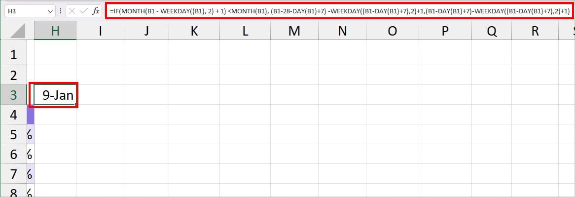
   
6. Then, I added the date by 7 (H3+7) in the second cell. I extended the Flash-Fill to have the data for the rest of the cells. If you get a #### error, select the cell range and enter Alt, H, O, I keyboard shortcut to fit texts.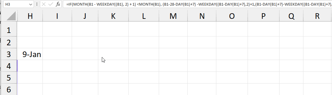
   
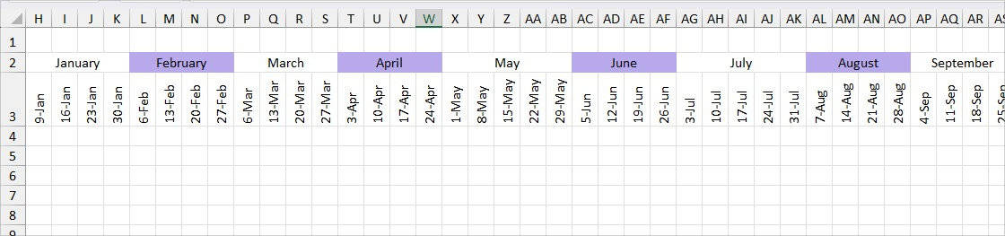
7. Type in the Month name just above the Date. You can apply Text Formatting to the Month name like Fill, Font, Bold, etc. For Dates, I changed the Text Direction to Rotate Text Up.
   

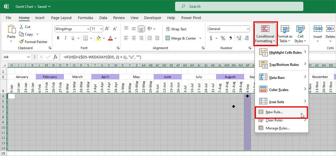
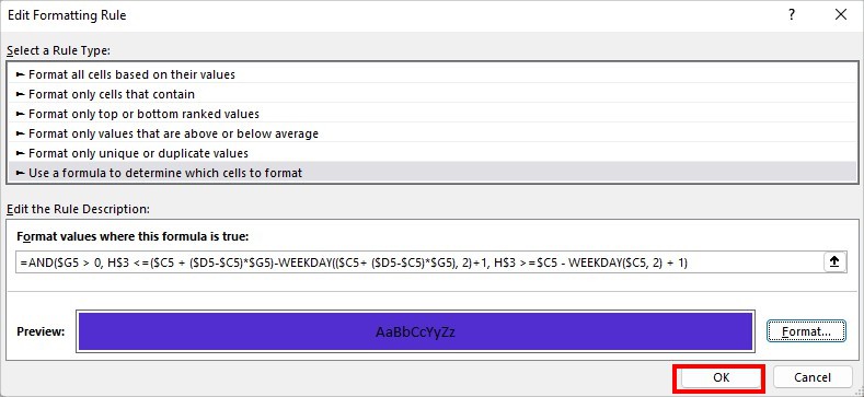
Step 2: Add Milestones

To add Milestones in the Gantt Chart that represent the End Dates, enter the given formula in the first date.

=IF(H$3=($D5-WEEKDAY($D5, 2) + 1), "u", "")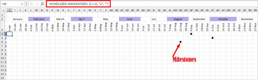

Change the Font Type to the Windings from the Home Tab. Now, use the Flash-Fill handle till the end to insert the milestones. When you do this, all the cell ranges will be empty. Only on the End date of the Task, you will have a Diamond character. 

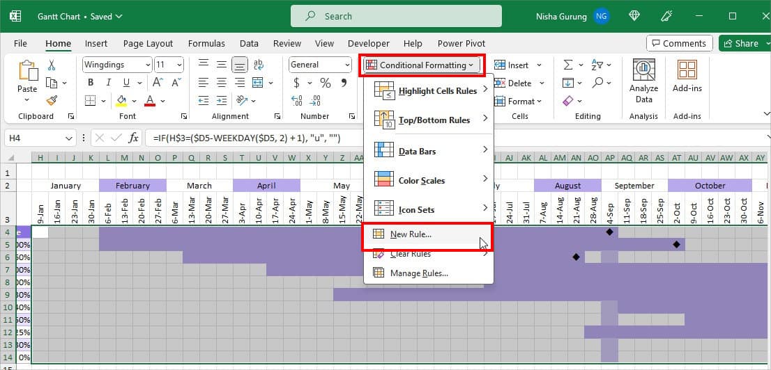
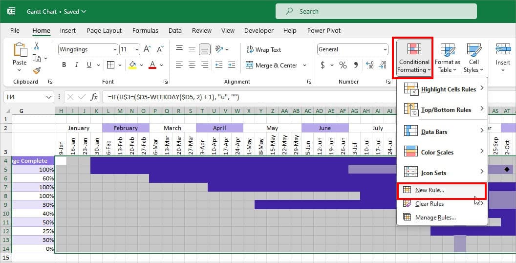
Step 3: Apply Conditional Formatting

1. Select the entire area of the Month.
2. From Home Tab, click on Conditional Formatting > New Rule.
   
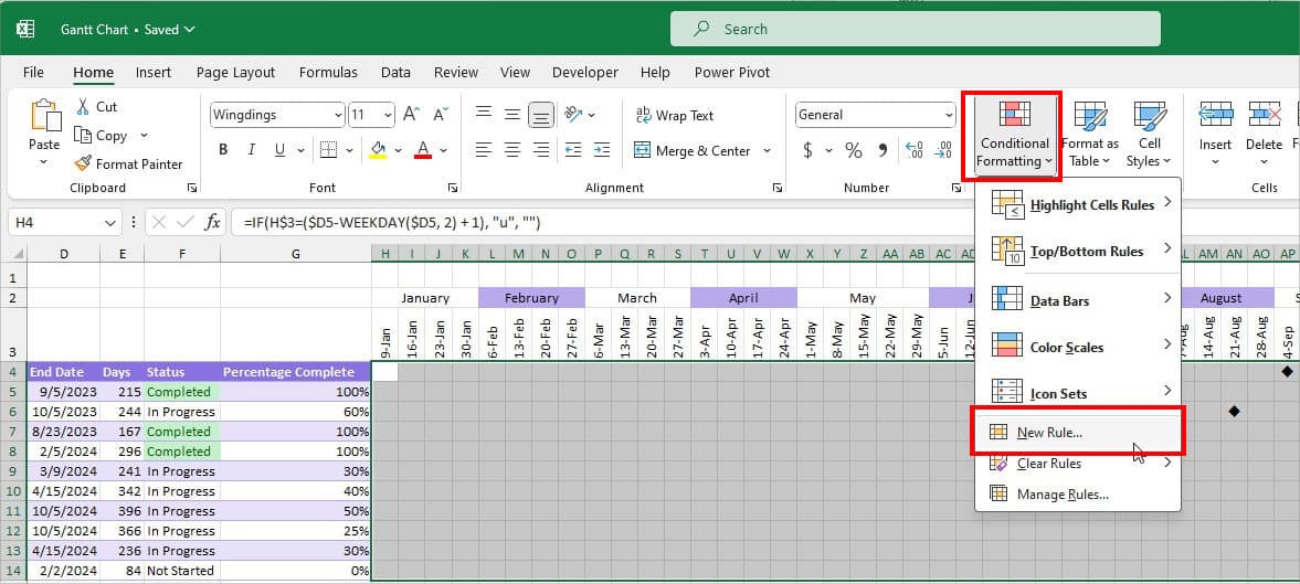
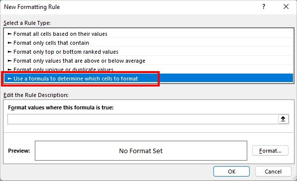
3. On the window, click on Use a formula to determine which cells to format below the Select a Rule Type.
   
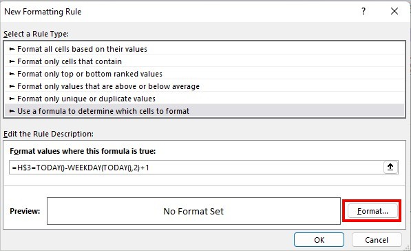
4. In the Format values where this formula is true, enter this formula =H$3=TODAY()-WEEKDAY(TODAY(),2)+1. Here H$3 is the first cell below the date to plot the Gantt Chart.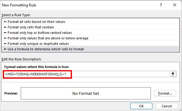
   
5. Click Format.
   
6. On Format Cells, head to the Fill Tab. Select a Colour and click OK.
   
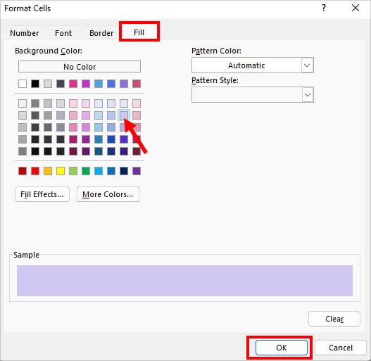
7. Click OK.
   

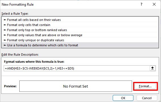
Step 4: Add Gantt Chart Bars

1. Select the area.
2. Choose Conditional Formatting > New Rule.
   
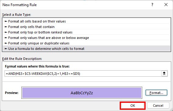
3. Select Use a formula to determine which cells to format. Then, enter this formula in the =AND(H$3>$C5-WEEKDAY($C5,2)+1,H$3<=$D5) field. (Here, H$3 is the first cell range to create Gantt Chart, and $C5 is first Start Date)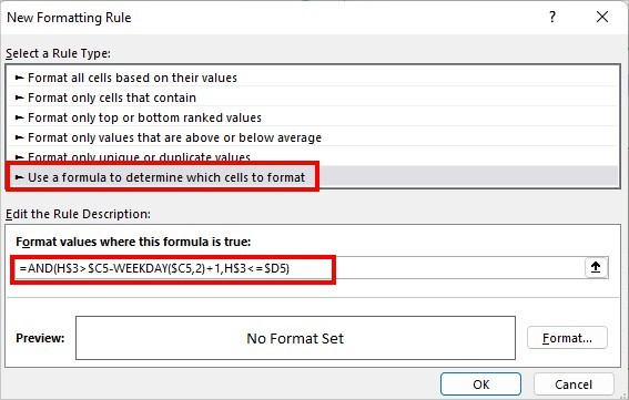
   
4. Hit Format.
   
5. From the Fill Tab, pick a Colour. Click OK. 
   
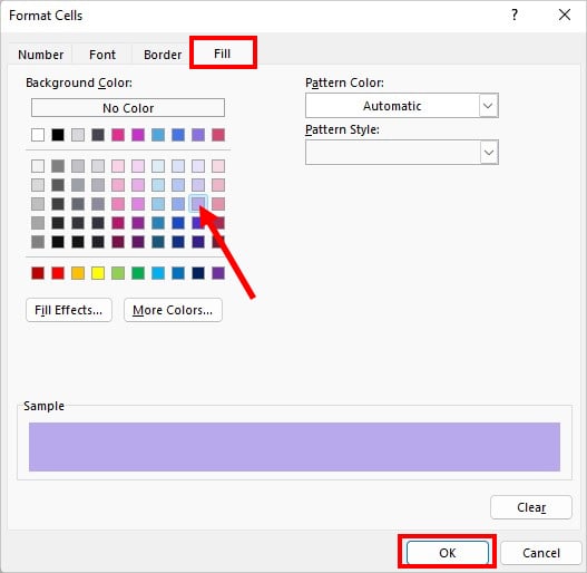
6. Hit OK. 
   

Step 5: Add Percentage Completed in the Gantt Chart

1. Select the Gantt Chart area.
2. Head to Conditional Formatting and click on New Rule.
   
3. Go to Use a formula to determine which cells to format and enter this formula =AND($G5 > 0, H$3 <=($C5 + ($D5-$C5)*$G5)-WEEKDAY(($C5+ ($D5-$C5)*$G5), 2)+1, H$3 >=$C5 - WEEKDAY($C5, 2) + 1). (Here, $G5 is the first percentage complete cell, $D5 is End Date, $C5 is Start Date)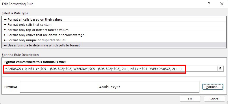
   
4. Click Format.
   
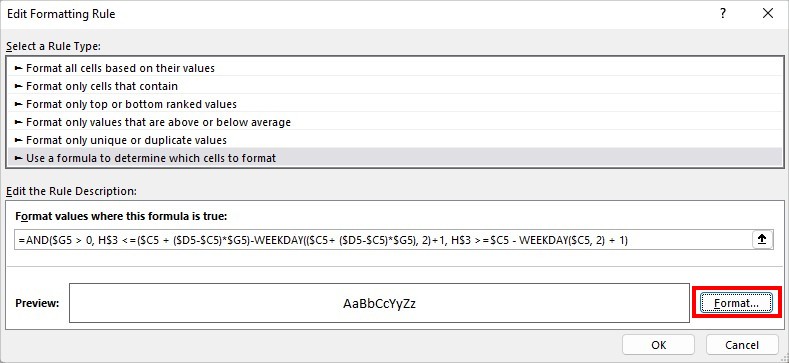
5. Choose Colour and click OK. I picked a Darker shade this time.
   
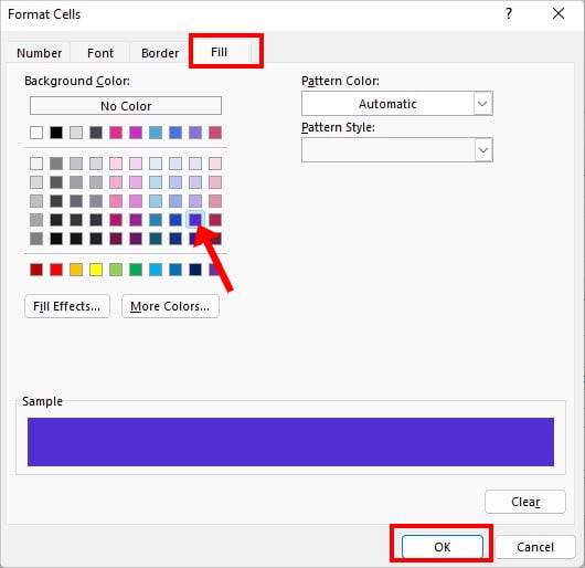
6. Hit OK.
   

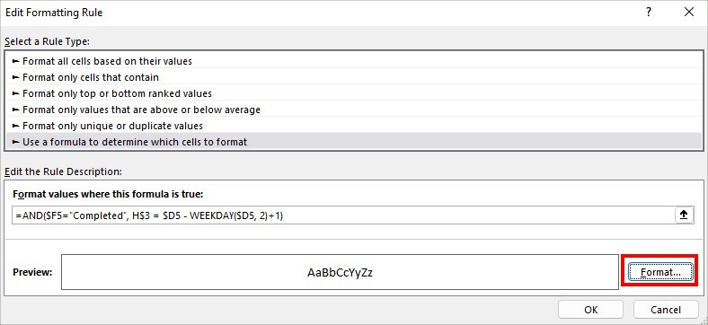
Step 6: Add Completed Status in the Gantt Chart 

1. Select Ranges and go to Conditional Formatting > New Rule.
   
2. Select Use a formula to determine which cells to format.  On the field, enter the formula =AND($F5="Completed", H$3 = $D5 - WEEKDAY($D5, 2)+1). (In the formula, $F5 is Status cell, $D5 is End Date)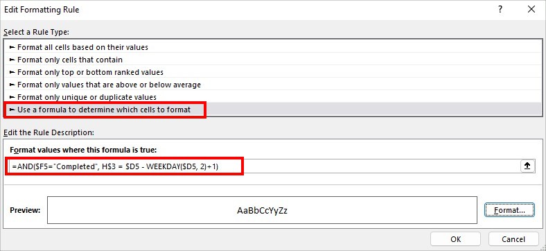
   
3. Click Format.
   
4. Pick a different Colour than the Gantt Chart bars and choose OK.
   
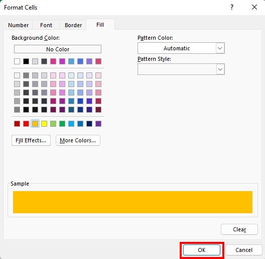
5. Hit OK.
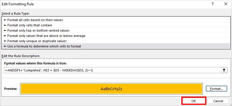
6. You’ll have a color for the Completed.