When you have many duplicate lookup_values in the lookup table, you must wonder whether you’d get the first, second, middle, or last occurrence as a return output.
Well, the truth is you can decide what match you wish to return for the lookup value.
In most lookup functions, the Exact Match returns the first occurrence by default. Similarly, if you need to return the last match from the lookup array, you can set Approximate Match in the formula argument.
However, in the case of the XLOOKUP function, you can actually determine the Search Mode to return the first or last occurrences.
Using VLOOKUP
To look up the first and last match in the VLOOKUP function, all you need to do is specify the range_lookup accordingly. Before we jump in with the examples, let’s recap the Function Syntax.
| Function Used | Syntax | Function Arguments |
| VLOOKUP | =VLOOKUP(lookup_value, table_array, col_index_num, [range_lookup]) | lookup_value: search value table_array: table or cell ranges to find the lookup value col_index_num: specify the column in table array to return the item. range_lookup: Enter logical value to specify how you want to search data. 1/TRUE: Approximate Match.0/FALSE: Exact Match |
Lookup First Match
In order to return the first match, your range_lookup argument in the VLOOKUP function should be FALSE or 0. In short, the exact match.
The formula will return the first match even if your data is not alphabetized or sorted.
Example:
In the lookup table, I have the Product, Estimated Sales, and Total Sales. In products, there are 3 duplicates for Coffee.
Let’s draw out the first occurrence.
Formula:
=VLOOKUP(F4,B5:D13, 3, FALSE)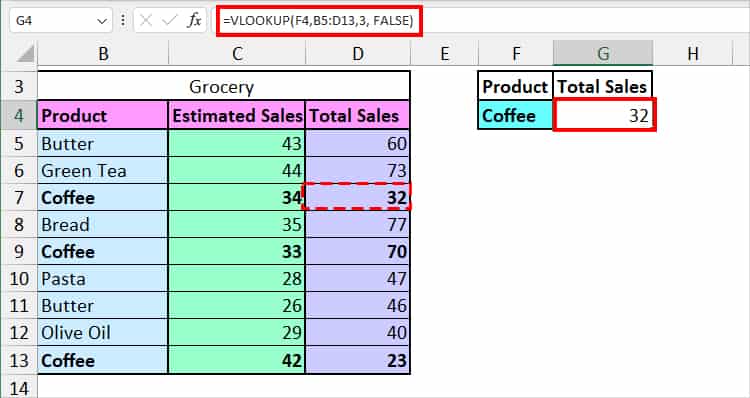
In the VLOOKUP formula, F4 is my lookup value. Since we have specified FALSE, the VLOOKUP returns the first exact match which is 32.
Lookup Last Match
To return the last lookup match, your range_lookup argument in the formula should be an Approximate match that is either TRUE or 1.
Also, to get the last match, you must sort or alphabetize your data first. Otherwise, the formula will result in the second or third occurrences from the lookup table instead.
Example:
Let’s return the final match from this A to Z sorted lookup table.
Formula:
=VLOOKUP(F4,B5:D13,3, TRUE)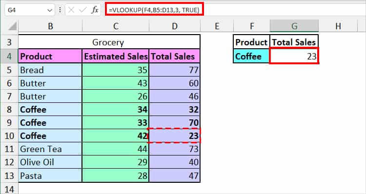
Since we have specified the TRUE argument, the formula will return the approximate match which is the last item in the lookup table.
Using INDEX and MATCH
INDEX and MATCH, a widely used duo lookup function, is one of the popular alternatives for the VLOOKUP function.
In case you use this function, here’s an example to look up start or end matches from the lookup table.
| Function | Syntax | Arguments |
| INDEX | =INDEX(array, row_num, [column_num]) | array: an array that has your value row_num: specify the row where your value lies column_num: specify the column where your item lies |
| MATCH | =MATCH(lookup_value, lookup_array, [match_type]) | lookup value: search item lookup_array: range where your lookup value lies [match_type]: determine match mode 1: Largest Match 0: Exact Match -1: Smallest Match |
Lookup First Match
When you need to return the first match using the INDEX and MATCH, specify your match_type as 0 (Exact Match) in the formula.
Before you start, make sure your columns are sorted.
Formula:
=INDEX(C3:C11, MATCH(F3, B3:B11, 0))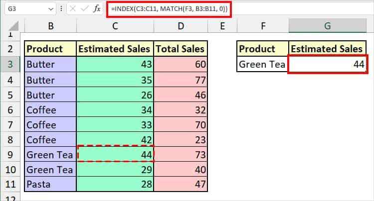
In the formula, the MATCH function returns the first position of the lookup value from the lookup array. Then, the INDEX function returns the value from the C3:C11 array which is 44.
Lookup Last Match
For the last item, your match_type should be 1 in the MATCH function.
Formula:
=INDEX(C3:C11, MATCH(F3, B3:B11, 1))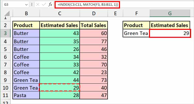
The formula resulted in 29 this time. This is because the MATCH function returns the last position of the lookup item. Similarly, the INDEX results in that corresponding value.
Using HLOOKUP
Similar to the VLOOKUP, the HLOOKUP function returns the first match when the range_lookup argument is FALSE and the last match when TRUE.
| Function | Syntax | Function Argument |
| HLOOKUP | =HLOOKUP(lookup_value, table_array, row_index_num, [range_lookup]) | lookup_value: value to search table_array: Array to find the lookup value row_index_num: specify the row in table_array to return the item from range_lookup: Boolean to return the match 1/TRUE: Approximate Match.0/FALSE: Exact Match |
Lookup First Match
Here, your range_lookup must be FALSE or 0.
Example:
From the data of Student and their French Marksheet, let us return the first score.
Formula:
=HLOOKUP("French", B3:E12, 4, 0)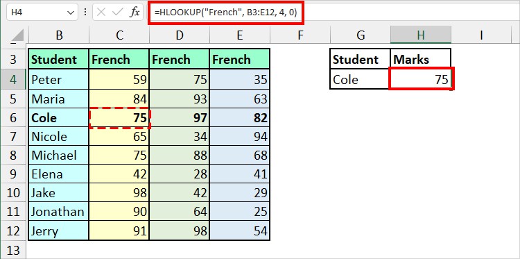
The HLOOKUP function returns the first occurrence from the fourth row for the French Lookup value.
Lookup Last Match
For the HLOOKUP to return the last match, the range_lookup argument must be TRUE or 1.
Example:
=HLOOKUP("French", B3:E12, 4, 1)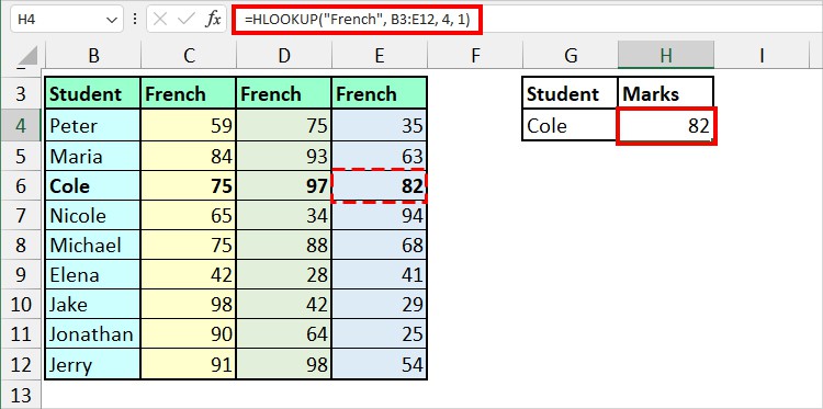
The formula now returns the last occurrence from the same row which is 82.
Using XLOOKUP
Compared to all the above lookup functions, the XLOOKUP function is the most advanced and powerful one.
Here, you can actually specify to return the lookup match from ascending, descending, first, and last in the Search Modes.
So, if you are using the XLOOKUP function, check out how to look up the first and last match.
| Function | Syntax | Function Arguments |
| XLOOKUP | =XLOOKUP(lookup_value, lookup_array, return_array, [if_not_found], [match_mode], [search_mode]) | lookup_value: Search Value lookup_array: table or range that has the lookup value return_array: Cell or ranges that you want to return from the lookup_array [if_not_found]: any text or item to return when there is no lookup value [match_mode]: Determine your lookup match 0: Exact Match -1: Exact or closest small item 1: Exact item or closest largest value 2: Wildcard Match [search_mode]: Choose how the order you want to search the value. 1: Search from start -1: Reverse Search that is from the last 2: Lookup items in ascending order -2: Lookup values in Descending order |
Lookup First Match
In the XLOOKUP function, you will get the first match when you specify 1 in the Search Mode. The best part is you do not have to arrange your data in any order.
However, if you want to return the first match in ascending or descending order, I would suggest you sort the lookup array.
Let’s return the first match for Butter lookup value.
Formula:
=XLOOKUP(F4, B4:B12, C4:C12, "No Sales", 0, 1)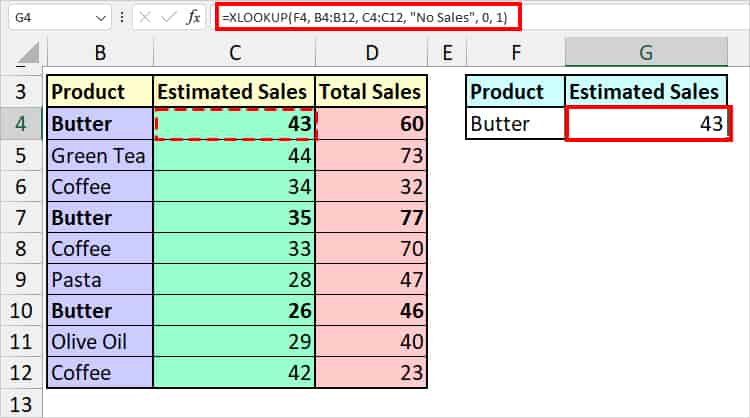
The above XLOOKUP formula returns the exact match from the C4:C12 column for the lookup value in F4 that lies in the B4:B12 column.
By entering 1 search mode, the formula will scan for the return array from the beginning and result in the first match. In case the lookup value isn’t there, I’d get No Sales.
The outcome is 43.
Lookup Last Match
Your Search Mode should be -1 to look up the last match. It reverses the search in bottom to top order and returns the first match.
In the same example as above, if I enter -1 as Search Mode, I’ll get the last item.
Formula:
=XLOOKUP(F4, B4:B12, C4:C12, "No Sales", 0, -1)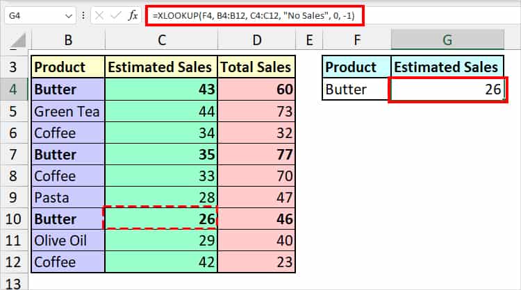
Since the XLOOKUP formula scans the return item from the last, I got 26 as a result this time.