As Google Sheets is a cloud-based spreadsheet, linking sheets isn’t as simple as compared to Excel.
To dynamically link sheets within the same workbook, you will have to create a formula specifying the sheet name and the range with your target data.
If the data you wish to link is in a completely different workbook, you will have to use the IMPORTRANGE function.
Before establishing a link, however, make sure you have the necessary permission to access the source spreadsheet.
Link Two Sheets Within Same Spreadsheets
To link sheets within the same workbook, you’ll have to construct a formula. The formula will consist of your sheet name and the range you want to link.
Our formula will follow the following syntax:
=(sheetname)!(cell)Take a look at this workbook.
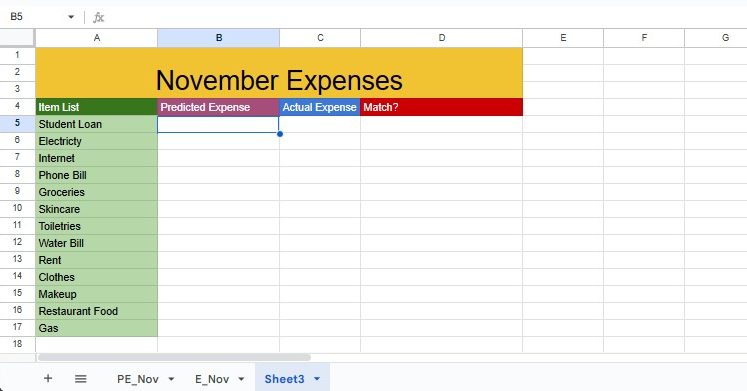
My workbook contains three sheets. The first sheet contains the budget I created for the month of November, and the second sheet contains my expenses for the same month. I want to pull data from both of these sheets to my third sheet.
In range B5:B17, I want to extract the predicted expenses, and in range C5:C17 I want to extract the actual expense.
In cell B5, enter the following formula to extract data from cell C4 in the first sheet, PE_Nov:
=PE_Nov!C4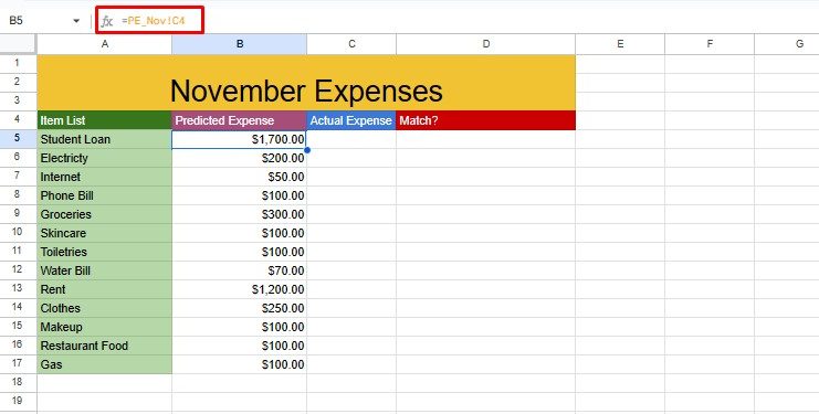
Similarly, in cell C5, I entered the following formula to extract data from cell C4 in the second sheet, E_Nov:
=E_Nov!C4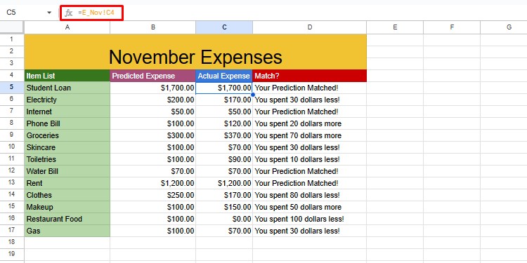
After that, use autofill to paste the formula to the entire column.
Link Two Sheets on Different Spreadsheets
| Function Used | Syntax |
IMPORTRANGE | =IMPORTRANGE(spreadsheet_url,range_string) |
If the data you want to link are in two different workbooks, you’ll have to use the IMPORTRANGE function to get data.
IMPORTRANGE is a pretty straightforward function. All you have to do is enter the source spreadsheet’s URL and reference the range with the data you wish to import.
You can also nest IMPORTRANGE with other functions when constructing formulas.
We’re creating a gradesheet in the following spreadsheet. I need to import the grades scored by each student for three subjects: Mathematics, English, and Science.
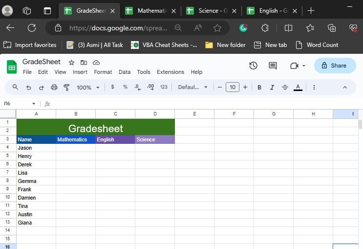
These data are however in three different workbooks. Here are the URLs to each workbook:
- Mathematics:
“https://docs.google.com/spreadsheets/d/1jN-RG4fLHcgz4OAwXirwk_Wkc-fNpg67wPemOwnh6hQ/edit#gid=0” - English:
“https://docs.google.com/spreadsheets/d/1GUjBX_4CWkE93-5iKSltPfrZu5eOGXZlpXEfu0Rs_KI/edit#gid=0” - Science: “https://docs.google.com/spreadsheets/d/1FLzs11rCyA8z0oFZu8dj3Ak5fGTwyBalhWcvkK7IoO0/edit#gid=0”
We will be pulling data from the F2:F11 range of all three spreadsheets. However, extracting data looks a bit different depending on the number of sheets inside the workbooks.
Let’s use IMPORTRANGE to make this arrangement.
If the Workbook Has Only One Sheet
The workbook containing the grades for Mathematics only has one worksheet. Therefore, we don’t have to specify the sheet name inside the IMPORTRANGE function.
In cell B4, I entered the following formula:
=IMPORTRANGE("https://docs.google.com/spreadsheets/d/1jN-RG4fLHcgz4OAwXirwk_Wkc-fNpg67wPemOwnh6hQ/edit#gid=0","F2:F11")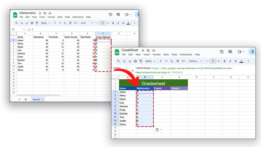
If Data is in the First Sheet
The book containing the grades for English has two sheets. However, as our data is in the first sheet, it isn’t necessary to include the sheet name in this scenario as well.
Here is the formula I used to import grades for English:
=IMPORTRANGE("https://docs.google.com/spreadsheets/d/1GUjBX_4CWkE93-5iKSltPfrZu5eOGXZlpXEfu0Rs_KI/edit#gid=0","F2:F11")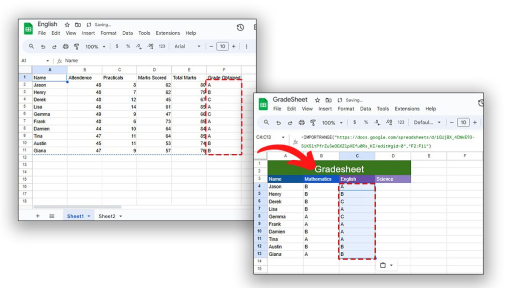
If Data is in the Second Sheet
In this case, the grades are on the second sheet of the workbook. Here, we must specify the sheet name for IMPORTRANGE to link data.
In cell D4, here is the formula I entered to import grades for Science:
=IMPORTRANGE("https://docs.google.com/spreadsheets/d/1FLzs11rCyA8z0oFZu8dj3Ak5fGTwyBalhWcvkK7IoO0/edit#gid=0","Sheet2!F2:F11")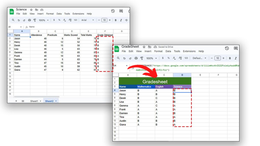
After entering these formulas, you will have to allow your current sheet to access information from the source sheet. Select the cell and click Allow access.
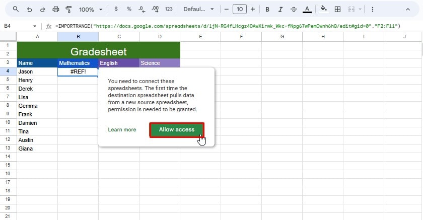
Once that’s done, Google Sheets will automatically load data from the source sheet.