How to Hide Zeros in Excel

As we perform various calculations, getting a resulting value like 0 is pretty normal in Excel. However, when they appear across all your worksheets, you might find these zeros quite unnecessary or rather distracting. Therefore, you may want to hide them to focus more on the actual data part. 

That said, we don’t want to accidentally remove zeros in numbers like 2001 or 1200. But, you might still want to remove leading/trailing zeroes in numbers like 001 and 2.00.

In that case, you need to set a custom formatting as mentioned in the article.

Using the Excel Advanced Options

Excel already has a built-in option that lets you hide cells with zeros. However, note that it affects the entire worksheet and not a particular cell range only.

1. Navigate to File > Options.
2. Select the Advanced tab from the sidebar.
3. In the right pane, scroll down to the Display options for this worksheet. If you have multiple worksheets, make sure you have selected the correct one in the dropdown next to it.
   
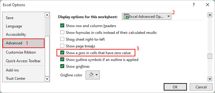
4. Now, under the same section, uncheck the Show a zero in cells that have zero value checkbox.
5. Click OK.

Using the Format Cells Option

Unlike the above method, you can hide zeros for both the selected cell range and across the whole worksheet. Here, we use a custom number formatting which will automatically hide any zero value as you enter it.

1. Select the cell range where you want to hide zero values.
   
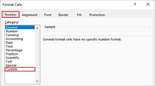
2. Then, press Ctrl + 1.
3. On the next prompt, click the Number tab and select Custom from the sidebar.
   
4. Now, replace General with 0;-0;;@ in the input field below Type.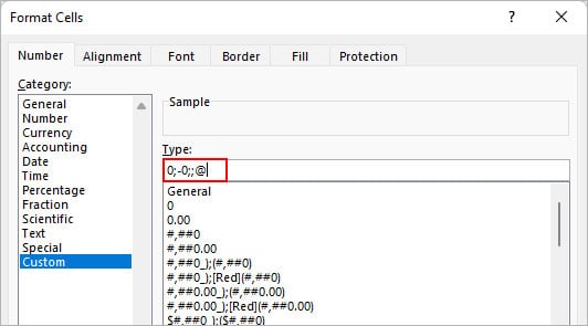
   

Using Conditional Formatting

Another way to hide zero is by using conditional formatting. Here, you filter all the cells with the “0” value and change their font color to white. Doing so will make the cell appear empty and get rid of all the cells containing the value 0.

1. Select the cells containing values as zero. Or, just select the cell range including such cells.
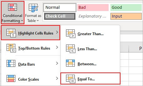
2. Under the Home tab, click Conditional Formatting and select Highlight Cell Rules > Equal to.
   
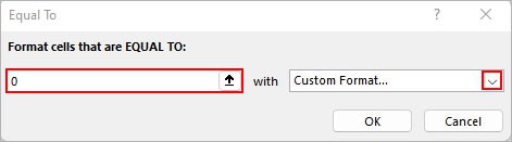
3. On the next prompt, enter 0 and select Custom Format from the dropdown menu.
   
4. Then, select the Font tab.
5. Under the Color section, choose white color.
   
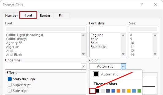
6. Click OK.

How to Hide Zero Values in an Excel Chart?

While Excel charts usually turn plain numbers into interesting visualizations, they rather appear quite messy when they display undesired zero values.

To remove the zero data labels from the chart,

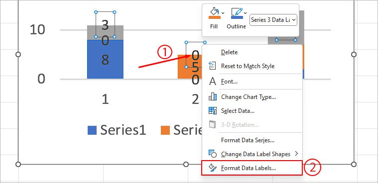
1. Select the data label with the zero value in the chart.
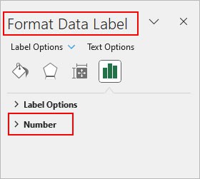
2. Right-click on it and select Format Data Labels.
   
3. Under the Format Data Labels sidebar, expand the Number dropdown.
   
4. Choose Custom under the Category section.
5. Under the Format Code section, enter #”” and click Add.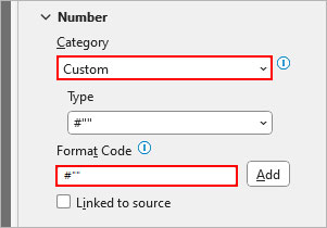
   
6. Repeat the same process to hide zeros for other data labels.

How to Remove Leading/Trailing Zeros in Excel?

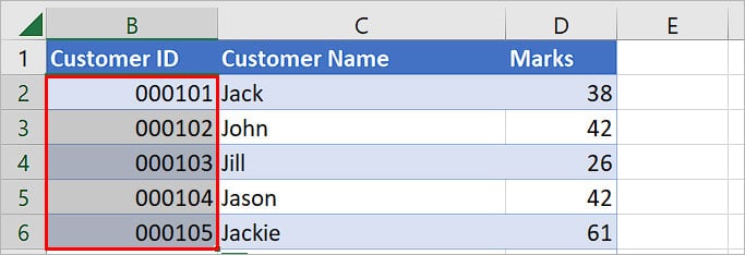
By default, Excel automatically hides the zeros in front of a number. However, if a cell is using custom formatting, you cannot simply delete those zeros.

On the other hand, if you are using a currency or accounting format, the trailing zeros usually appear at the end like $2.00.

In both cases, you would have to change the number formatting to get rid of zeros.

1. Select the cell range which contains extra leading zeros.
   
2. Press Ctrl + 1 to launch the Format cell window.
3. Then, click the Number tab and select Custom from the sidebar.
4. Under the Type section, choose the General option.
   
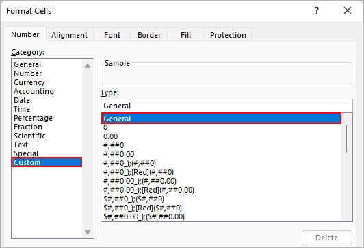
5. Click OK.
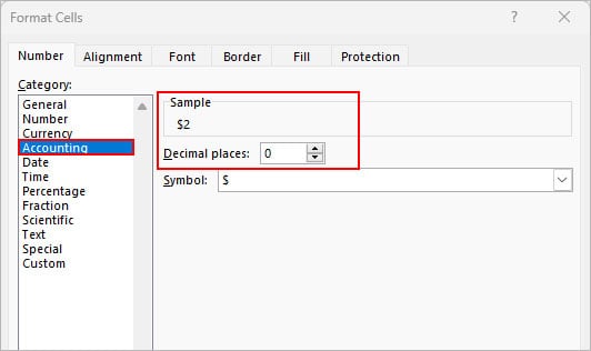
6. Similarly, to remove trailing zeros like in the number $2.00, select the cells with such numbers. Then, choose Currency or Accounting under the Category section and set the Decimal places to 0.
   

How to Replace a Cell Containing “0” with a Dash Symbol?

While all the above methods hide zero values, sometimes it can get confusing if you just leave them like that. So, you could rather replace them with a character like a dash to represent blank cells.

To find cells with only 0 and not some other value like 20,

1. Select the cell (s).
2. Press Ctrl + H to open the Find and Replace window.
3. Then, type 0 next to Find what field. Also, enable the Match entire cell contents.
   
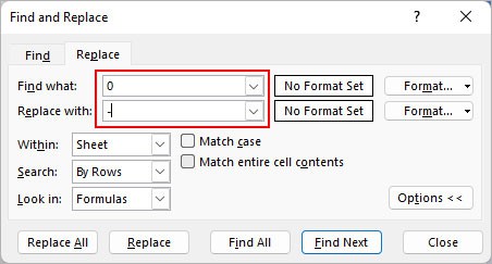
4. Enter a dash character next to the Replace field. Alternatively, you can enter another preferred character as well.
5. Click Find Next to review which cells are being affected.
6. Click Replace All.