As a rookie in digital marketing, I used to manually count the total number of sales while calculating relative frequency in Excel. Spoiler alert: I almost always made the wrong count!
However, this was before I discovered functions in Excel. While there isn’t a dedicated function that calculates the relative frequency of range, you can use the COUNTIFS and the SUM functions to make this calculation.
Talking from personal experience, this method is not only faster than manually calculating relative frequency but is also mostly foolproof.
How to Find Relative Frequency in Excel
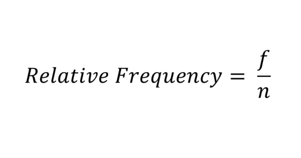
Let’s start with the formula of finding the relative frequency first. Assuming,
f = Frequency
n = Total Frequency
Relative frequency is calculated to see what portion of the selected frequency covers the total frequency. It is mostly calculated to compare the occurrences during data analysis.
In Excel, you can use the COUNTIFS and SUM functions to find the relative frequency of a range. The COUNTIFS function will count the occurrence of each frequency while the SUM function will calculate the total frequency of each occurrence.
We will then use the divide operator (/) to compute the relative frequency using each of these values.
Step 1: Use COUNTIFS to Cout the Frequency
We will be using the COUNTIFS function as we will be needing to pass two criteria to make a count. If you’re not as familiar with the COUNTIFS function in Excel, here is how the function is written in as a formula:
=COUNTIFS(criteria_range1, criteria1, [criteria_range2], criteria2)For more details about this powerful function, I highly suggest you check out this article I covered on how to use COUNT and COUNTIFS functions in Excel.
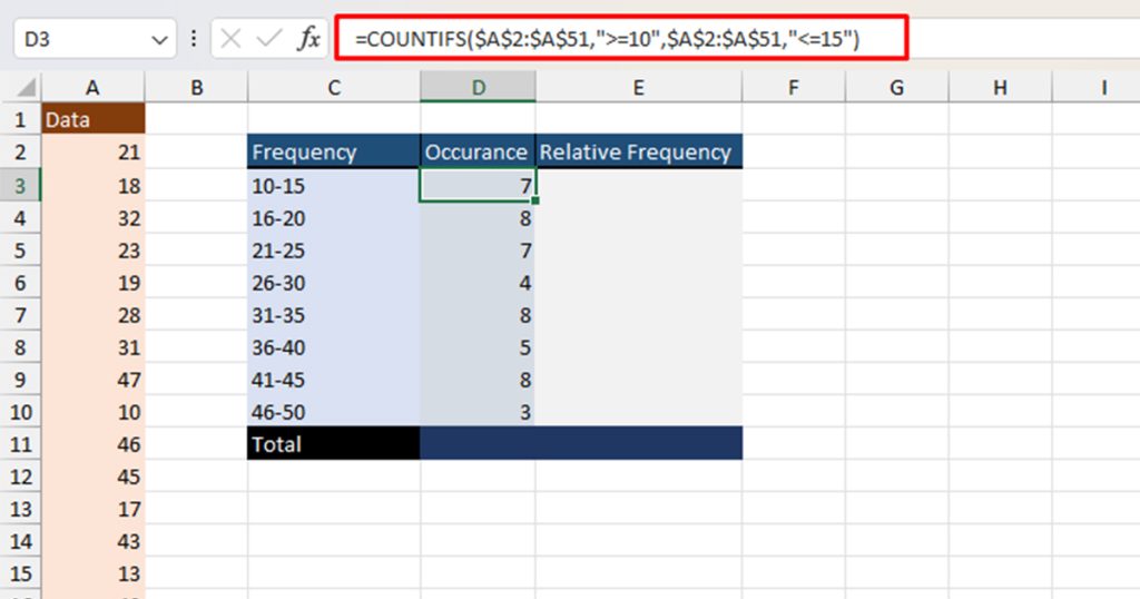
Let’s put this function to use. Here we have a table in range A2:A51 with data ranging from 10-50. We have made a second table with our frequencies. Here’s the formula I applied to count each of these frequencies

| Frequency | Formula Used | Result |
| 10-15 | =COUNTIFS($A$2:$A$51,">=10",$A$2:$A$51,"<=15") | 7 |
| 16-20 | =COUNTIFS($A$2:$A$51,">=16",$A$2:$A$51,"<=20") | 8 |
| 21-25 | =COUNTIFS($A$2:$A$51,">=21",$A$2:$A$51,"<=25") | 7 |
| 26-30 | =COUNTIFS($A$2:$A$51,">=26",$A$2:$A$51,"<=30") | 4 |
| 31-35 | =COUNTIFS($A$2:$A$51,">=31",$A$2:$A$51,"<=35") | 8 |
| 36-40 | =COUNTIFS($A$2:$A$51,">=36",$A$2:$A$51,"<=40") | 5 |
| 41-45 | =COUNTIFS($A$2:$A$51,">=41",$A$2:$A$51,"<=45") | 8 |
| 46-50 | =COUNTIFS($A$2:$A$51,">=46",$A$2:$A$51,"<=50") | 3 |
Step 2: Calculate the Total Frequency Using SUM
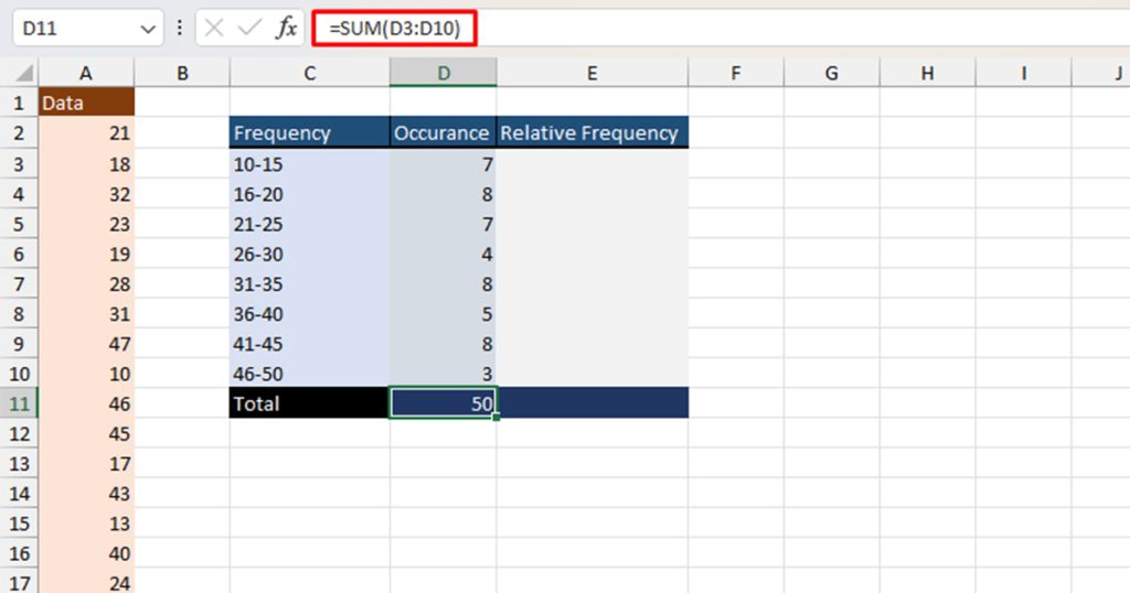
Now, we will be adding up the counts we made using the COUNTIFS function. While you can also use the + operator to add these values, I prefer using the SUM function for larger values. This is because SUM takes arrays as an argument while I will have to individually reference each cell with the operator in between using the + operator.
The SUM function is written in the following way when putting it into a formula:
=SUM(range)=SUM(cell1,cell2,cell3)We will be using the first way to add all of our values in the range. This is the formula we used:
=SUM(D3:D10)
Step 3: Divide Each Frequency By the Total Frequency
After calculating the total frequency, you can finally head on to calculating the relative frequencies. To make this division, we will be using the “/” operator which essentially performs division. The value you enter before the / operator is treated as the numerator while the value that follows is the denominator.
This is how you can use the “/” operator while constructing a formula:
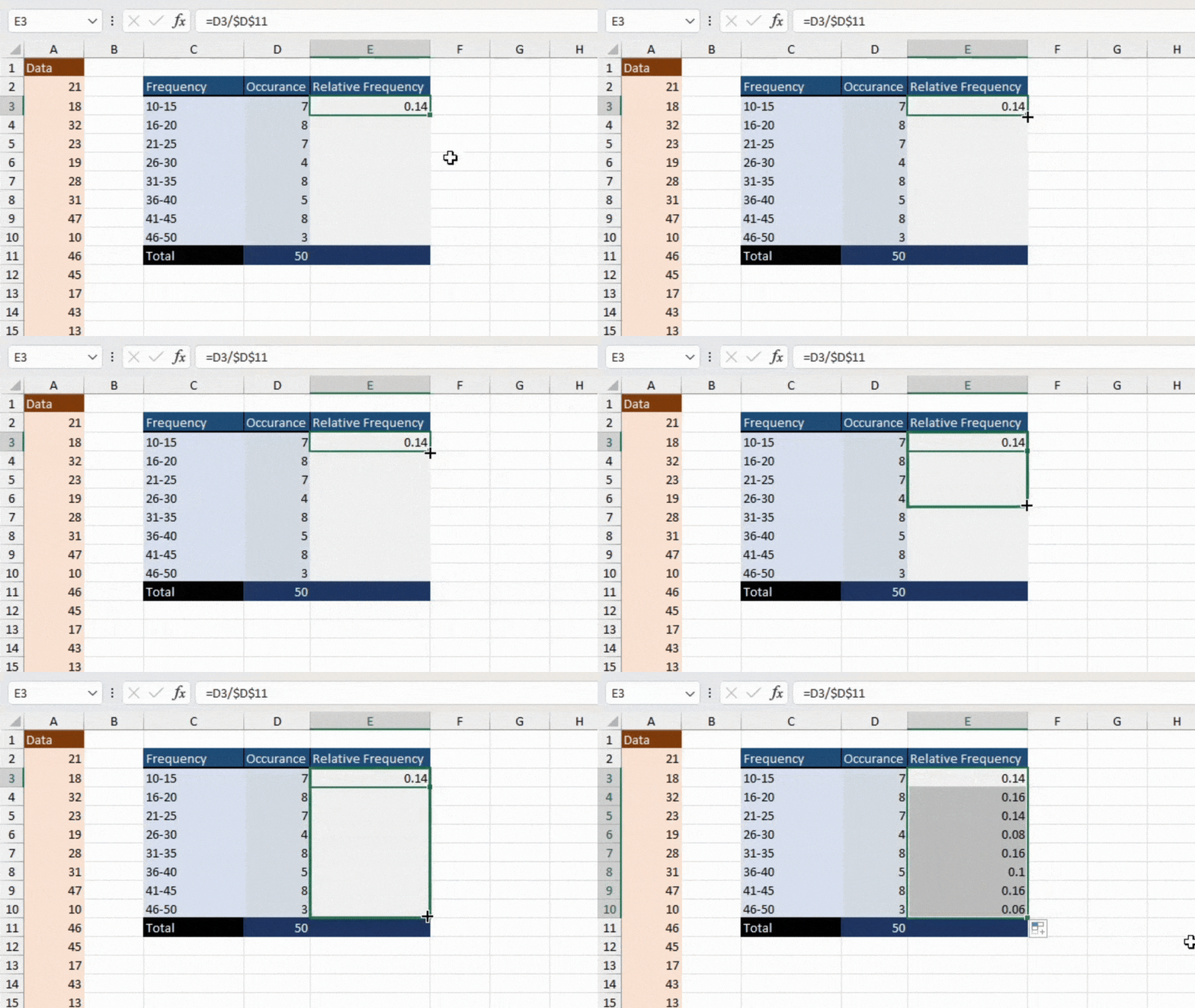
=(numerator)/(denominator)I first divided cell D3 which holds the occurrence of values from 10-15 in the range by cell D11, the total frequency. Then I simply copied the formula using the flash fill feature onto the remaining cells.
Here’s the formula I applied using the “/” operator to calculate the relative frequency of these values:
=D3/$D$11