How to Create Drop-down List on Excel

Rather than manually entering data in individual cells, you can create a dropdown list in Excel to populate cells with pre-defined options. Along with providing the options, you can also display a message to warn users whenever they try to enter a non-valid option.

You can create various dropdown lists based on the comma-separated delimiter, cell range, named range, and table. Also, you can store them in a different worksheet so that the users can focus on the input only.

To create one,

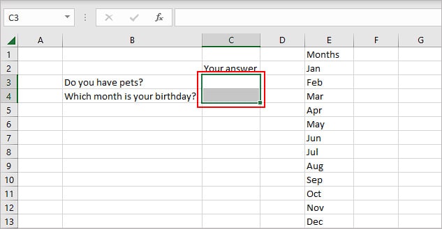
1. Select the cell (s) where you want to insert the list.
   
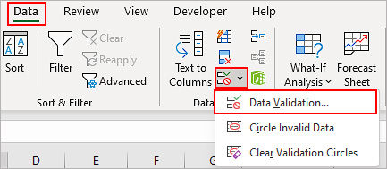
2. Select Data validation under the Data tab.
   
3. Click the Settings tab.
4. Under the Allow section, select the List option.
   
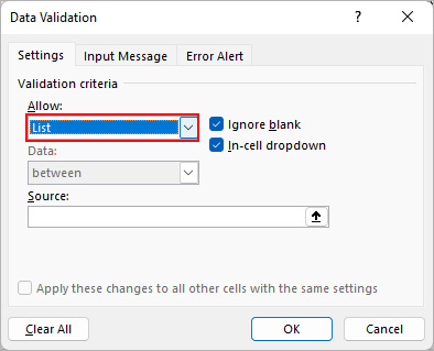
5. Disable the Ignore blank checkbox to warn users from leaving the cell empty while selecting it. However, if nothing is selected by default on the cell and it’s already empty, the user doesn’t get displayed any message.
6. Enable the In-cell dropdown checkbox.
7. Click the Up arrow icon under the Source section.
   
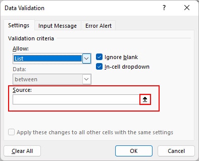
8. Now, choose one of the following methods.
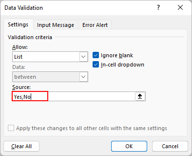
   • Comma Separated Delimiter: This method is particularly useful if you only have a few options like Yes/No, and True/False. Here, you manually enter the options separated by a comma.
     
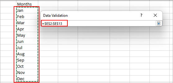
   • Cell range: Here, you simply drag across the cells which you want to include as options.
     
   • Named range: Instead of manually entering or selecting the cell reference of the dropdown list options, you can name such a cell range. Then, you can enter the name instead of the whole cell reference in the source section.
     
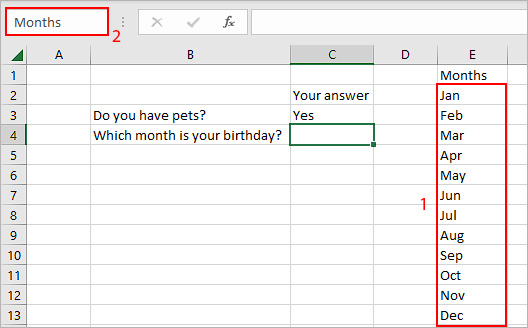
     To name a cell range, type the desired name in the name box located at the top-right corner of the window.
9. Click OK.

Quick Tip: Consider placing the dropdown list options in a separate sheet so that the user can focus on the cell input rather than the list.

How to Create a Dropdown List Based on a Table?

While the above two methods mentioned in Step 2 do a decent job of creating a dropdown list, a better approach is to create one that’s based on tables. The benefit of such dropdown lists is that whether you need to add or delete any of the list values later, the table updates them automatically. This means every cell based on that list will have new options.

To create a list based on the table, 

1. First, you need to convert your dropdown list values into a table. So, navigate to the worksheet containing the list of options. Then, select them and press the Ctrl + T shortcut. 
2. On the Create Table window, click the Up arrow icon and select the cells containing the options. Enable the My table has headers checkbox if the options column contains a header and click OK.
   
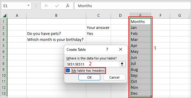
3. Additionally, you can even provide a named range for the list. To do it, select the cell range with options and provide a name in the name box.
   

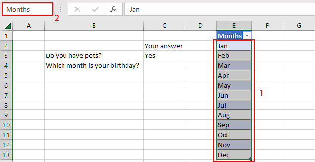
How to Display a Message while Selecting the Cells with Dropdown Values?

While creating a dropdown list, you can even display a message to inform what the list contains and what they are expected to enter.

1. Select the Input Message tab. 
2. Then, enter the preferred message. 
3. Additionally, select the Show input message when the cell is selected option to display the message when the active cell contains the dropdown list.
   

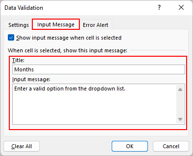
Similarly, you can alert a user when trying to enter a different option as follows:

1. Select the Error Alert tab and enter the error message you want to display. 
   
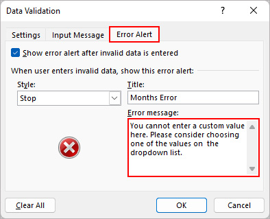
2. Also, enable the Show error alert after invalid data is entered checkbox.

How to Protect the Dropdown List Data?

If you don’t want others to edit your list options, you can protect the cells containing the dropdown lists. Surprisingly, all cells in a worksheet are locked by default on Excel.

So, you first have to unlock the cells you want others to be able to edit, which in our case is choosing a dropdown option. Then, protect the worksheet with a password to only select unlocked cells.

1. Select the cell range with dropdown lists and any other cells you want the users to edit.
   
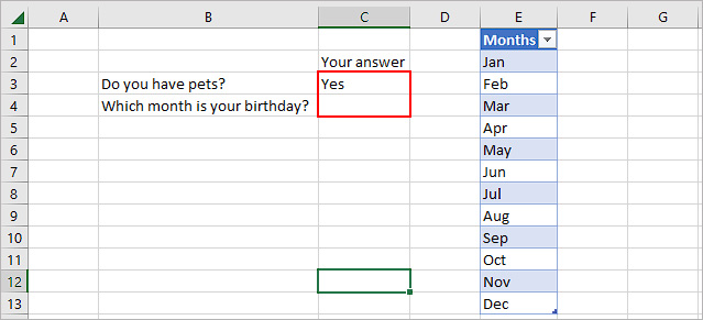
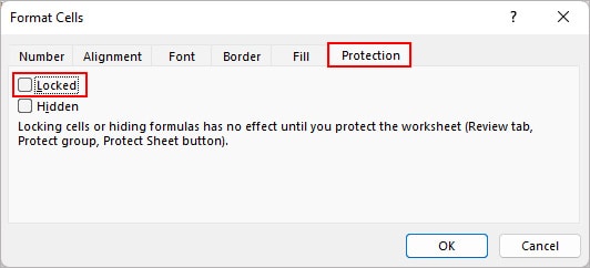
2. Press Ctrl + 1 to open the Format cells window and select the Protection tab.
3. Uncheck the Locked checkbox and click OK.
   
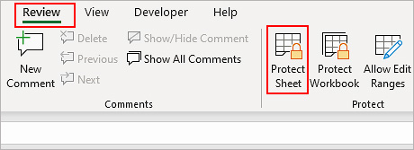
4. Then, under the Review tab, click Protect Sheet.
   
5. Enable Select unlocked cells and disable Select locked cells checkboxes.
   
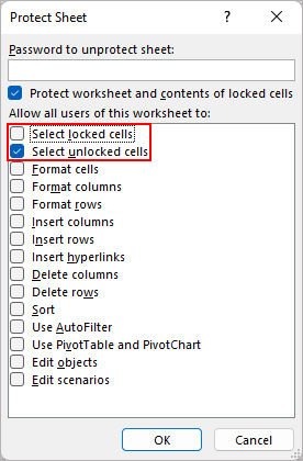
6. Enter a password and note it somewhere safe as you have to use it to unprotect the sheet and edit the contents.
   
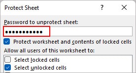
7. Click OK.

To unprotect the sheet,

1. Select the Review tab and click Unprotected Sheet.
   
2. Use the password you set earlier when asked.

How to Create a Dependent Dropdown List?

While working with multiple dropdown lists, you may sometimes come across a situation where options selected on one list determines what options to display on another one. 

In such cases, you need to create a dependent dropdown list.

For instance, you have two dropdown lists among which one contains the laptop names. And, depending on the laptop, you have to create another list showing the respective laptop models.

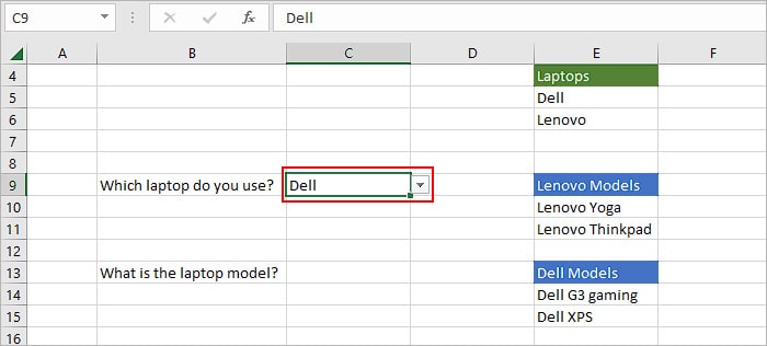
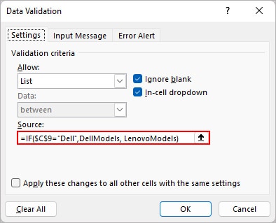
Here, the C9 cell contains the first dropdown list asking for the name of the laptop with two options; Dell and Lenovo. And, we have two names ranges among which DellModels include Dell G3 and Dell XPS. Similarly, the name range LenovoModels includes Lenovo Yoga and Lenovo Thinkpad.

Here, we need to create a dependent dropdown list so that when the user chooses Dell for “Which laptop do you use?”, they only get options under the Dell Models. Similarly, if they choose the Lenovo option, they can choose options under the Lenovo Models.

To create a dependent dropdown list, you can use the simple IF function.

1. Create the first dropdown list with options for laptop names. 
2. Next, you need to create the dependent dropdown list to show the laptop model options based on the laptop name.
3. Select the cell where you want to create the dependent dropdown list. Here we are using the C13 cell.
   
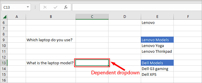
4. Go to Data > Data Validation.
5. Under the Source section, use the IF function.
   =IF($C$9="Dell",DellModels,LenovoModels)