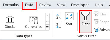
As you apply a filter, Excel hides the rest of the data except the filtered cells. So, only the cells containing the filtered data are visible.
However, sometimes when you try to copy only the filtered results, the rest of the data (non-filtered and hidden cells) also show up while pasting. On top of it, they might not even end up in the respective rows/columns.
In such cases, you can use Excel’s built-in tools like Go To and Advanced Filter, which help to select or directly copy the filtered values only.
- Ctrl + Shift + Down arrow: To select all the filtered values in a single column.
- Ctrl + Shift + Right-arrow: To select the filtered values in a single row.
Using the Go to Feature
The Go to feature contains a special option that only selects the filtered cells. Additionally, it also excludes any other hidden cells.
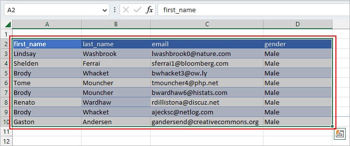
After using it, you can see a whitish border around cells, suggesting that Excel is only selecting the filtered cells.
- Select the filtered cells you want to copy.
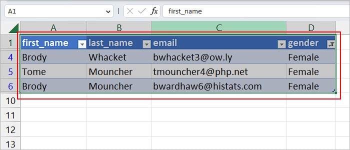
- Press Ctrl + G.
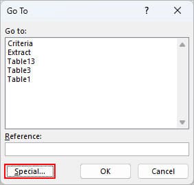
- On the next prompt, click Special.
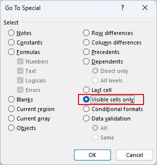
- Then, select the Visible cells only option and click OK.
- Press Ctrl + C to copy them. If you are using Mac, use Command + C shortcut instead.
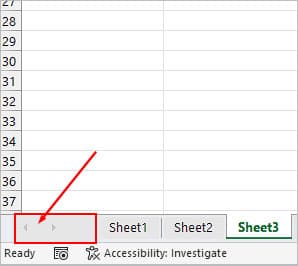
- To paste them into another worksheet, right-click between the two arrows icon on the left side of the Sheets tabs.
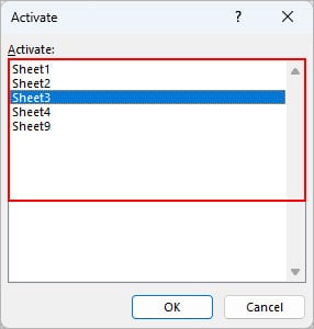
- On the Activate prompt, select the Sheet you want to paste the data and click OK.
- Now, simply paste (Ctrl + V) the data in the preferred cell location of the new worksheet.
Using Advanced Filter
Along with the filter options you get on the column header, Excel also has an additional advanced filter feature.
Not only does it filter based on the specified criteria, but it also provides an option to instantly copy and paste the results within the same worksheet.
- Select the cells where you want to apply the filter.
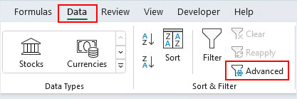
- Under the Data tab, click the Advanced option. Look for it in the Sort & Filter section.
- On the next prompt, choose the Copy to another location option.
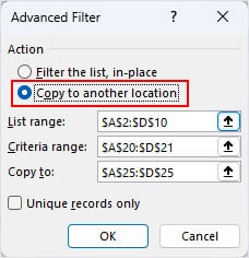
- Enter the cell range for the following fields. Use the Up arrow icon to select the cell range.
- List range: Cell range of the dataset you want to apply the filter
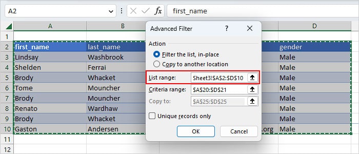
- Criteria range: Cell range containing your criteria. Here, we are filtering cells with first_name= “Brody” and last_name= “Whacket”.
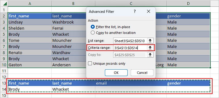
- Copy to: Cell range where you want to copy and paste the filtered results
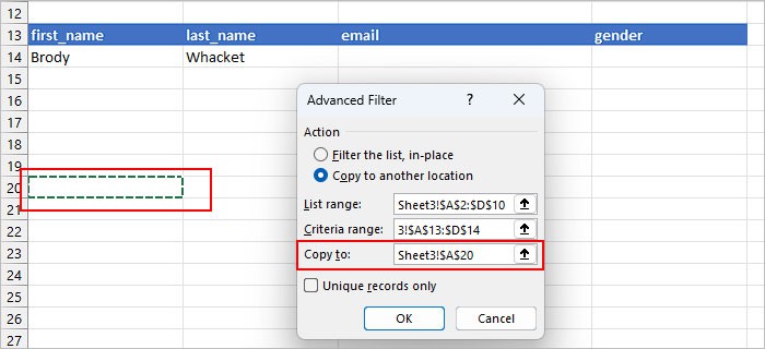
- List range: Cell range of the dataset you want to apply the filter
- Additionally, enable the Unique records only checkbox to filter out unique records among the filtered data.
- Click OK.
Related Questions
How to Unhide Non-Filtered Results?
While it may appear that the non-filtered results have vanished or been deleted, they are actually hidden. After copying the filtered data, you can retrieve them as follows:
- Click the column header where a filter is applied. You can see a little funnel icon next to the header on such columns.
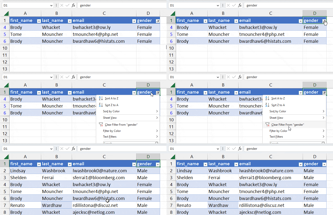
- Then, select Clear filter from <column name>.
- Alternatively, go to the Data tab and click Filter to disable it.
