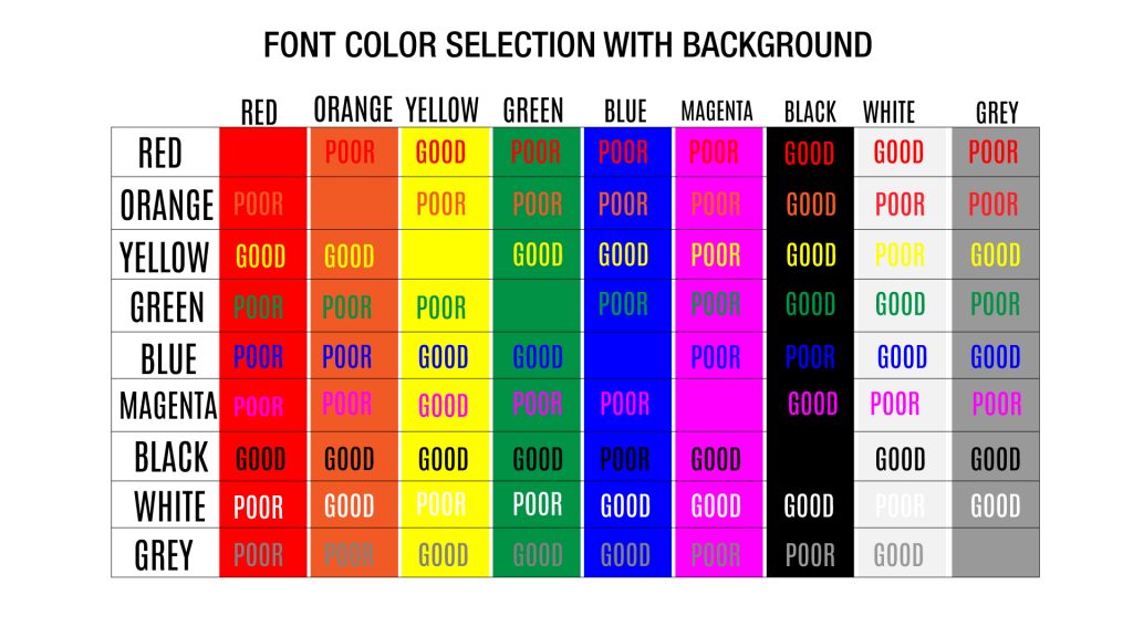
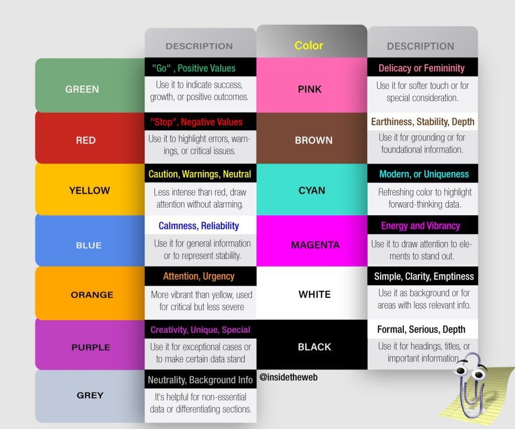
Naturally, we associate colors with emotions. For example, we associate numbers colored red with danger and green with safe. You can incorporate such color coding to represent your data visually.
You may be looking to color-code your data for a number of reasons. When preparing a sales sheet, you can represent profit as green, loss as red, and breakeven as yellow.
If your data is smaller, you can manually shade your cells as your preferred color. However, if your data set is extensive or dynamic, you’re better off using Conditional Formatting in Excel.
Manually Color Code Data
If you’re looking to color code a few pieces of data in the spreadsheet that follows no particular rule, you can simply fill the cells with color in them.
- Select your cell or range.
- Go to the Home tab.
- Select the fly-out next to the fill bucket in the Font tab.
- Choose a color.
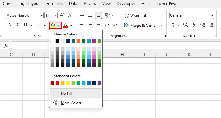
- For more color options, select More Colors > Choose a color > OK.
Apply Rule for Color Coding
In Excel, you can set a formatting rule using the Conditional Formatting tool. If you use Excel for basic data analysis, you probably can use one of Excel’s rules that are already available in the program. You can set your own custom rule for more advanced color coding.
Once you’ve specified a rule, you have to choose a format. Excel will apply the set formatting on the cell/range that matches your criteria. You can either apply a solid color or even format your range to follow a color scale.
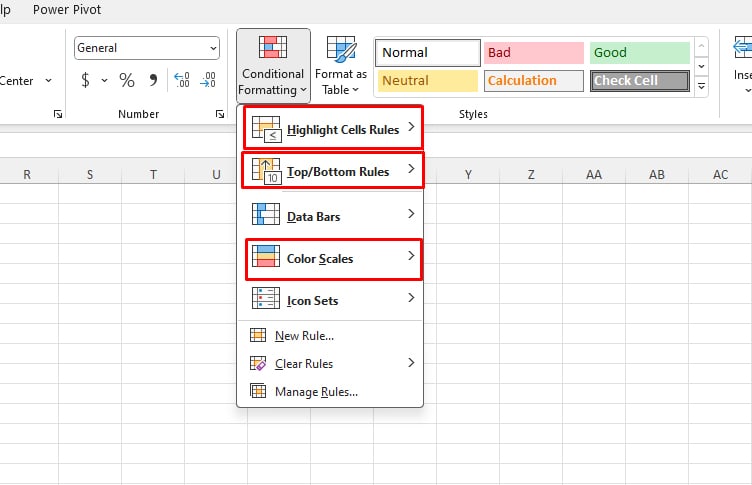
Here are some of the built-in rules you can use to color code your values in Excel:
- Highlight Cells Rules
- Top/Bottom Rules
- Color Scales
Color-Code Specific Data
You can use the first, Highlight Cells Rules option to color-code specific data. This option allows you to color code your value according to the following rules:
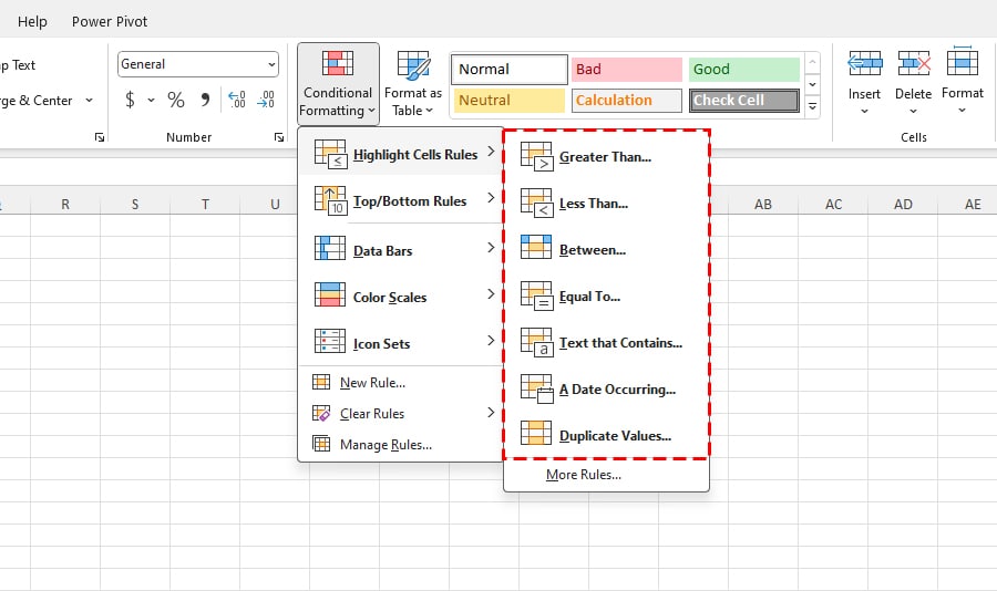
- Greater Than: Color cells that are greater than a set number.
- Less Than: Apply color to cells that are less than a set number.
- Between: Color code cells that fall under the specified range.
- Equal To: Fill cells that have the exact number.
- Text that Contains: Color-code cells that contain a specific text.
- A Date Occurring: Color-code according to dates.
- Duplicate Values: Highlight duplicate values.
Example
In this example, I’ll be color-coding data that falls between the range of 0-40.
- Select your data range.
- Go to the Home tab and select Conditional Formatting from the Styles section.
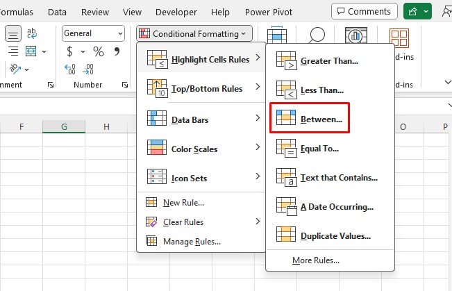
- Choose Highlight Cells Rules > Between.
- Enter the bottom figure on the first input box. In our case, this is 0.
- In the next input box, enter the maximum number. This is 40 in our case.
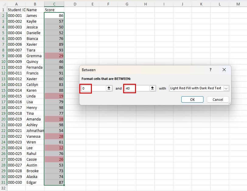
- In the next section, select the fly-out to choose a format.
- Click OK.
Color-Code Top/Bottom Data
The next Excel rule, Top/Bottom rules color-codes the top and bottom values in Excel. This Excel option is limited to only numeric values. Here are the rules Excel offers in color-coding top/bottom rules:
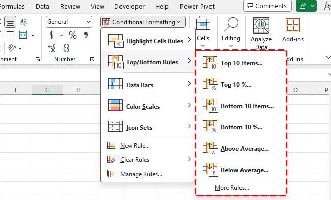
- Top 10 Items: Color 10 cells that have the highest numbers.
- Top 10 %: Highlights the numbers that take the top 10% of the range. This data is generated by dividing the number by the range’s total.
- Bottom 10 Items: Shade 10 cells that have the lowest numbers.
- Bottom 10 %: Colors the cells with numbers that take the bottom 10% of the range.
- Above Average: Highlights cells that are above the calculated average.
- Below Average: Highlights cells that are below the calculated average.
Example
Let’s color code values in the top 10% range using the Top/Bottom Rule.
- Select your data set.
- Head to Home and select Conditional Formatting.
- Click on Top/Bottom Rules.
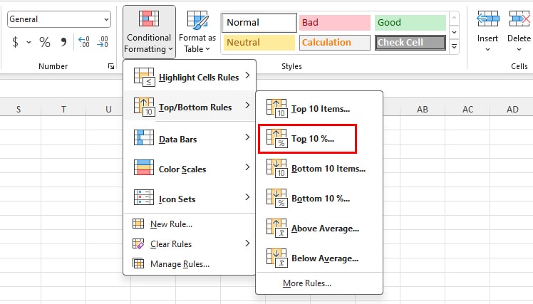
- Next to ‘with’, choose a format.
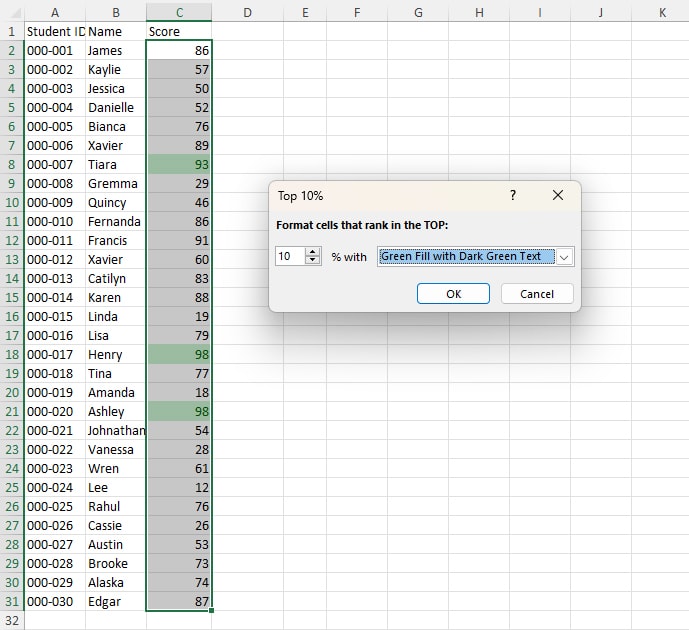
- Click OK.
Color-Code Numbers in a Scale
If you want to color each data in your cell according to its hierarchy, you can choose the Color Scales option. Just as color-coding top/bottom rules, you can only use the Color Scales option in numeric values.
Excel will present you with a few presets for this option. However, you can customize the gradient from the More Rules option.
Example
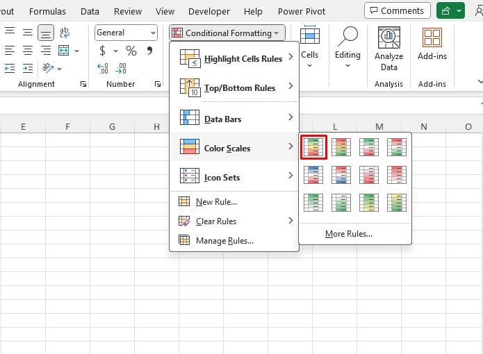
We will be color-grading our data to mark the lower ones with shades of red, the average with shades of yellow, and the higher ones with shades of green.
- Select your data range.
- From the Home tab, click on Conditional Formatting.
- Choose Color Scales.
- Select the Green-Yellow-Red Scale.
Set a Custom Color-Coding Rule
If you wish to color code your values using a custom formula, you can create a New Rule. In this rule, you can enter a formula. Excel will apply the set formatting on those cells that match the criteria of the specified formula.
Example
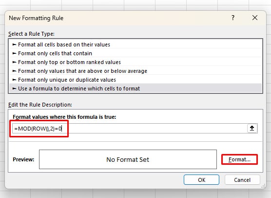
Let’s create a formula that will color-code every other row in our data set.
- Select your range.
- Go to Home > Conditional Formatting > New Rule.
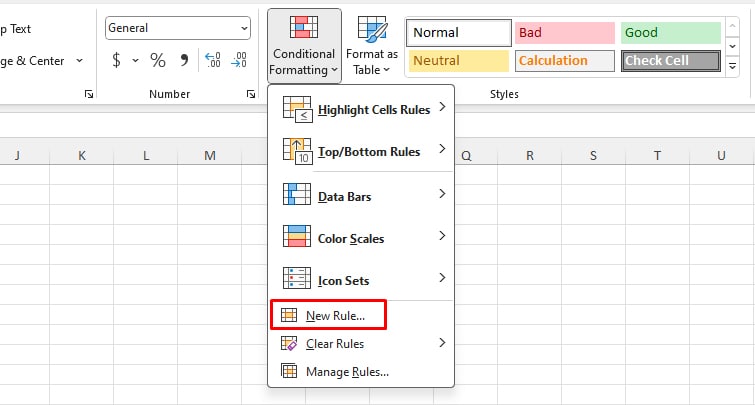
- Under Select a Rule Type, choose Use a formula to determine which cells to format.
- Enter your formula under Format values where this formula is true. In our case, our formula will be:
=MOD(ROW(),2)=0- Click Format to select a formatting.
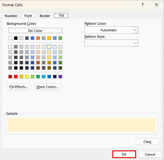
- Switch between the Border and Fill tabs and select a color.
- Click OK > OK.
Best Font Colors for Background
When choosing the right font color, it is essential that you match the color with the background. The background and foreground color should be distinct, not blend with each other, easy for your eyes and look professional at the same time.
