Whenever you use a formula for calculation, Excel displays it in the (fx) Formula bar by default.
While it is extremely helpful to track the cell references and functions used, Excel offers its users to control the appearance of these formulas. Meaning, you can hide or unhide them anytime you want.
Method 1: Hide Formulas From the Cell
If you’ve enabled the Show Formula option, formulas will appear in cells instead of values like in the given picture.

To hide these formulas and display only the values, you can disable this feature. For this, navigate to Formulas Tab. Then, on the Formula Auditing section, click on Show Formulas to disable it.

Alternatively, there is also an Excel shortcut key to easily show or hide formulas. If you prefer shortcuts, enter the following keys together.
Shortcut: CTRL + `Method 2: Hide Formulas From the Formula Bar
Whenever I’m sharing my Excel spreadsheets with clients or colleagues, I make sure to always lock and hide formulas. I wouldn’t want other users to mess with the formulas I’ve used in the data as even the slightest change can lead to a #### error.
If you also want to retain your data integrity, I suggest you use this method. Along with hiding formulas, here, you are protecting all the cells with formulas as the users cannot edit the formula cell.
Step 1: Unlock Cells
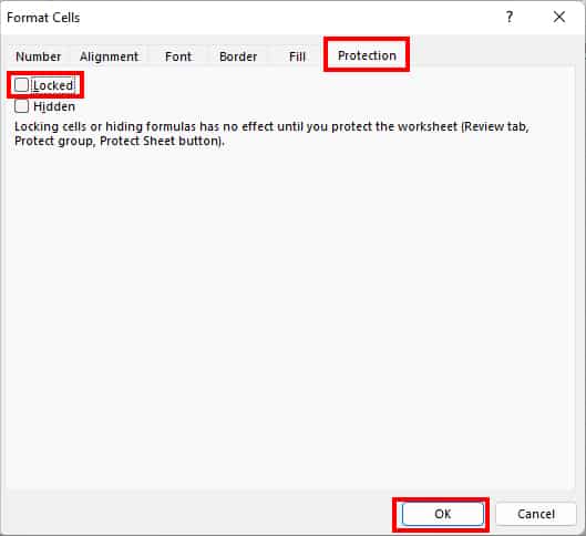
Firstly, you’ll have to unlock the cells in order to lock them. This is because Excel already locks them by default. But, note that even if the Locked menu is ticked on the Protection tab, the effect applies only after protecting your worksheet.
- Click on an empty cell and press Ctrl + A to select all cells.
- Press Ctrl + 1 key to bring up Format Cells window.
- Head to Protection Tab. Untick the box for Locked and click OK.
Step 2: Lock and Hide Formula Cells
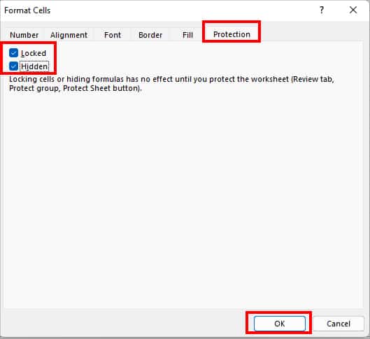
Now that we have unlocked all cells above, here we will specifically lock only formula cells. Also, this is a crucial step as we need to tick the options for both Locked and Hide while locking cells.
- Select the formula cell ranges.
- Enter Ctrl + 1 for the Format Cells window.
- Click on Protection Tab. Tick the box for both Locked and Hidden.
- Then, click OK.
Step 3: Protect Sheet
Finally, in the third step, we will protect the worksheet to completely hide and lock the formula cells. While protecting the sheet, you can even keep passwords and selectively share them with certain people only.
- On your spreadsheet, navigate to Review tab.
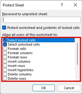
- From the Protect group, select Protect Sheet.

- Below Allow all users of this worksheet to, tick the options to allow users to format.
- Then, in the Password to unprotect sheet box, type a Password to lock the formula cells with. (Optional)
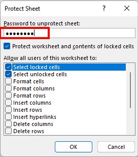
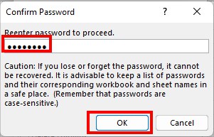
- If you kept the password, Re-type the password to verify and click OK.
Method 3: Hide Formula Bar
Suppose, you’re showing your spreadsheet to other users on your PC itself. To prevent them from viewing the formula, you can put away the formula bar temporarily.
Other than restricting users, this method also comes in handy when the formula is huge and takes up a lot of space. To do so, navigate to View Tab on your worksheet. Then, from the Show group, untick the Formula Bar option.

If you’ve to keep switching between showing and hiding the Formula Bar, we recommend you use the given shortcut keys. Note that you do not have to press all keys at once. As it is Excel’s ribbon shortcut, you can press down the keys one by one like Ctrl. Then, Alt, and so on individually.
CTRL + ALT + V + F