Gridlines are basically horizontal and vertical lines that spread across rows and columns. Excel displays them by default so that it’s easier to identify each cell in the worksheet.
However, if your worksheet contains design elements like a chart or a dashboard, you may want to hide gridlines for better visualization.
On Excel, you can hide/show gridlines across an entire worksheet or workbook. And, while you can’t do so for a particular area of a worksheet, you can still use cell borders as an alternative solution.
Using the Excel Advanced Options
Using the Excel Advanced options, you can show/remove gridlines for the worksheet(s) or even a whole workbook. Also, you can apply the gridlines setting for multiple worksheets at once.
- Select File > Options.
- Click the Advanced tab.
- Scroll down to the Display options for this worksheet section.
- Click the dropdown next to it and select a whole workbook or one of the worksheets for which you want to show/hide gridlines.
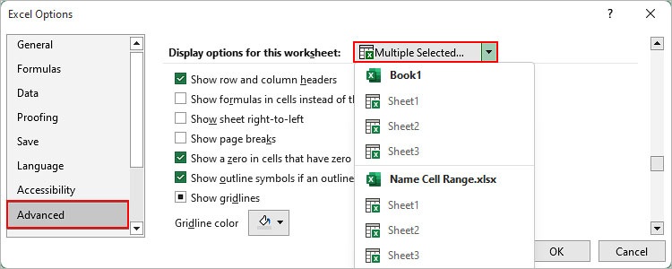
- Then, uncheck the Show gridlines checkbox to hide or enable it to show gridlines.
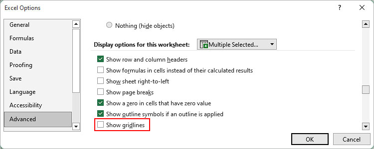
- To select multiple worksheets in a workbook, first select them while pressing the Ctrl key. Then, repeat the above steps and make sure you choose the Multiple Selected dropdown worksheets option.
Using the Page Layout Tab
You can also use the Page Layout tab to quickly show/remove the gridlines on your worksheet.
- Select the Page Layout tab.
- To hide/remove the gridlines, disable the View checkbox under Gridlines. You can find it inside the Sheet Options section.

- Similarly, enable the View checkbox to show gridlines.
Using the View Tab
Another way to show/hide gridlines is through the View tab.
- Select the View tab.
- To hide/remove the gridlines, uncheck the checkbox next to Gridlines inside the Show section.

- To show it again, enable the Gridlines checkbox.
Via the Quick Access Toolbar
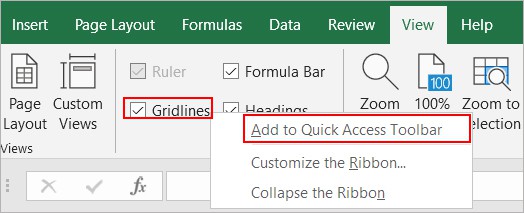
Initially, you don’t have gridlines on the quick access toolbar. However, you can add the gridlines setting much like other Excel tools. Once you do so, you can easily access them no matter which tab you are using.
- Go to the View tab.
- Right-click on Gridlines and select Add to Quick Access Toolbar.
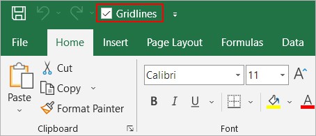
- Now, the Gridlines setting should appear at the top left corner and you can enable/disable its checkbox to show/hide it.
How to Show or Hide Gridlines for a Specific Region in a Worksheet?
Whether you turn on or off gridlines, Excel reflects it on the whole worksheet. Now, this can sometimes become an issue if you want to display gridlines for specific data only and leave other spaces blank.
To solve it, you can use cell borders as an alternative. Here’s how to do it.
- First, turn off the gridlines. Then, select the region where you want the gridlines.
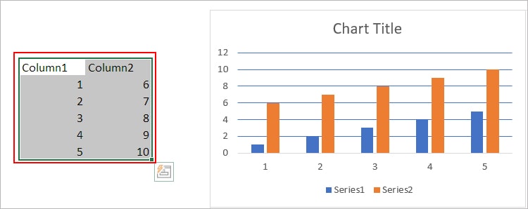
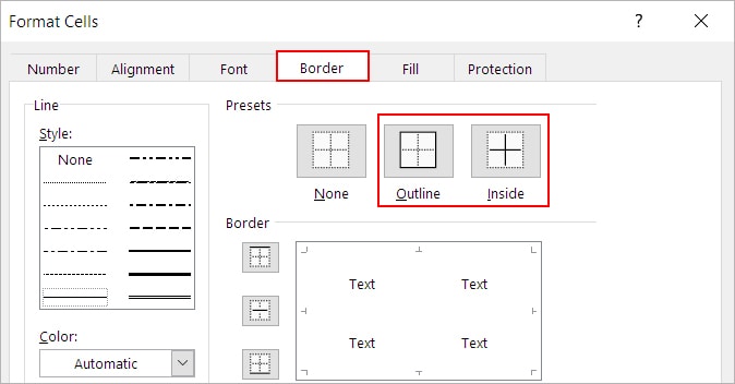
- Now, you need to apply a cell border. So, press Ctrl + 1 and select the Outline/Inside option under the Border tab. Additionally, use the color gray if you want it to appear as regular gridlines.
Note: By default, tables will display cell borders even if you hide gridlines.How to Enable or Disable Gridlines for Charts?
Some charts come with built-in gridlines inside them. To disable gridlines on them,
- Select the chart.
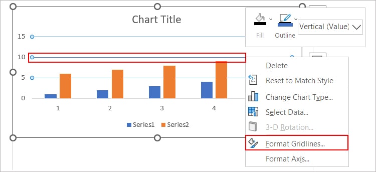
- Right-click on one of the gridlines and select the Format Gridlines option. Or, select anywhere on the chart area and select the Format Plot Area option.
- Once the navigation pane appears on the right side, expand Line/Border and select No line to hide the gridlines inside the chart.
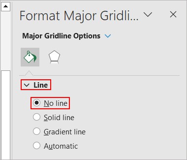
- To enable gridlines, choose other options like the Solid line and Gradient line.
How to Show Gridlines while Printing?
By default, the gridlines don’t appear when you print the worksheet. However, you can choose to show them on the printed paper as follows.
- Select the Print Layout tab.
- Enable the Print checkbox under Gridlines.

Related Questions
Why Am I Still Seeing the Gridlines Even after Disabling Them?
If you see some dotted lines across your worksheet, they aren’t actually gridlines, but probably automatic page breaks or cell borders. So, you need to disable/remove them instead.