The IMPORTRANGE function is an exclusive function in Google Sheets to link data from different sheets. If you usually merge data between sheets, you may need to familiarize yourself with this function.
IMPORTRANGE is dynamic in nature—every time you edit the source sheet, the change is immediately reflected on the linked data.
Using this function, you can not only create links between multiple worksheets but also append data.
Now, let’s first start with the arguments used in this function.
IMPORTRANGE Function: Arguments
=IMPORTRANGE(“spreadsheet_url”, “range_string”)- Spreadsheet_url: The Uniform Resource Locator (URL) of your source spreadsheet
- Range_string: The sheet and range name containing the data you wish to source
After entering the formula, you will first encounter the #REF error as your sheets aren’t currently connected.
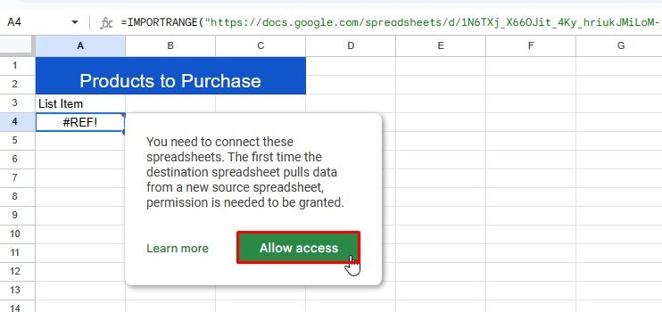
To fix this, select the cell with the formula and click Allow Access.
Link Data When Workbook Contains Single Sheet
If your workbook contains only one sheet, you don’t necessarily have to specify the sheet name. Simply referencing the range will do the trick.
The following workbook contains only one sheet.
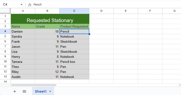
We’ll be importing data from range C4:C13 from this sheet. In cell A4 of the destination sheet, I entered the following formula:
=IMPORTRANGE("https://docs.google.com/spreadsheets/d/1N6TXj_X66OJit_4Ky_hriukJMiLoM-_nYFu-1lbBMcU/edit#gid=0","C4:C14")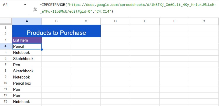
Link Data When Workbook Contains Multiple Sheets
You must specify the sheet’s name if the source workbook contains multiple worksheets. If you skip this, IMPORTRANGE will import data from the first sheet in the workbook.
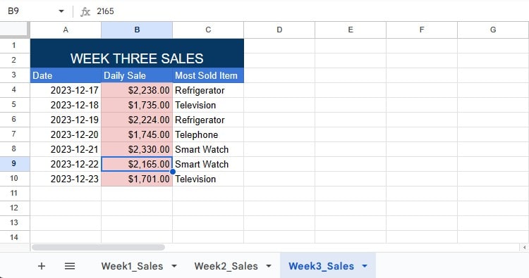
The following workbook contains three sales sheets. However, I only want to import data from range A4:B10 in the third worksheet, “Week3_sales”.
In my destination worksheet, I entered the following formula to make this extraction:
=IMPORTRANGE("https://docs.google.com/spreadsheets/d/1N6TXj_X66OJit_4Ky_hriukJMiLoM-_nYFu-1lbBMcU/edit#gid=1216284927","Week3_Sales!A4:B10")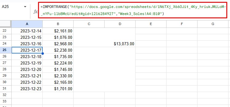
Append Data from Multiple Worksheets
You can also use the IMPORTRANGE function to stack data from multiple worksheets onto each other.
This workbook contains two worksheets.
On a new workbook, I want to stack data from Sheet2 on top of Sheet1.
For this, I will be creating an array formula using the IMPORTRANGE function.
Here’s the formula I entered to make this arrangement:
={IMPORTRANGE("https://docs.google.com/spreadsheets/d/118L0nmqG0nDYifB95LCGFhDjkOKjb5hqyxAhtZC2Ay8/edit#gid=0","Sheet1!A3:F17");IMPORTRANGE("https://docs.google.com/spreadsheets/d/118L0nmqG0nDYifB95LCGFhDjkOKjb5hqyxAhtZC2Ay8/edit#gid=0","Sheet2!A4:F17")}
When you enclose a formula inside curly brackets, you’re commanding Google Sheets to treat it as an array formula. If you do not enter the curly brackets, it will return the #ERROR code.
Use IMPORTRANGE Dynamically
You can reference cells as arguments inside the IMPORTRANGE function. For instance, if cell A2 contains the sheet URL, I can simply reference the cell inside the spreadsheeet_urlsection of the IMPORTRANGE formula.
Every time I change the values inside the referenced cells, IMPORTRANGEwill generate a different result, making the formula dynamic.
We can further incorporate Data Validation in the referenced cell to create a drop-down list.
Here’s how you can use the function dynamically in GSheets:
- Select an empty cell in your workbook.
- Click on Data > Data Validation.
- From the sidebar, select Add Rule.
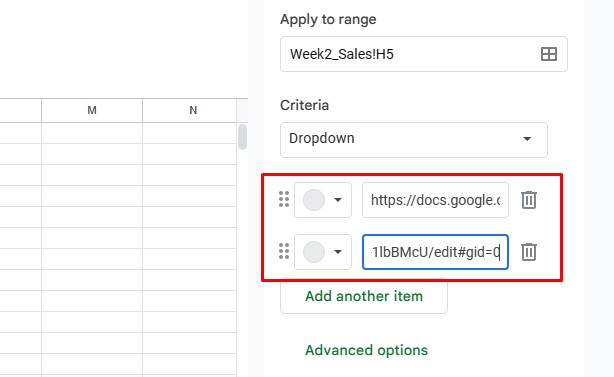
- Enter your URLs in the Option section. To add more options, click on Add another item.
- Select OK.
- Select Add Rule again.
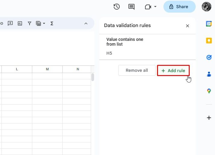
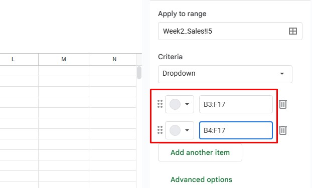
- Repeat this to create a drop-down list for the cell ranges.
- Enter your formula into the cell in which you wish to import your data.
=IMPORTRANGE(H4,I4)- To change your data set, click on the drop-down and choose a URL. Specify the cell range accordingly.
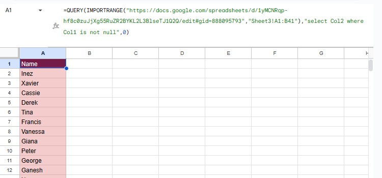
Set Criteria Using Query in IMPORTRANGE
If you want to set conditions while importing data, use the QUERY function with IMPORTRANGE.
The QUERY function can be a bit complex as it uses a specific language. Refer to Google’s article on this language to better understand the syntax to set criteria.
As an example, we have a data table with a list of students appearing for an exam. Unfortunately, only the students with a registration number are allowed to sit this exam.
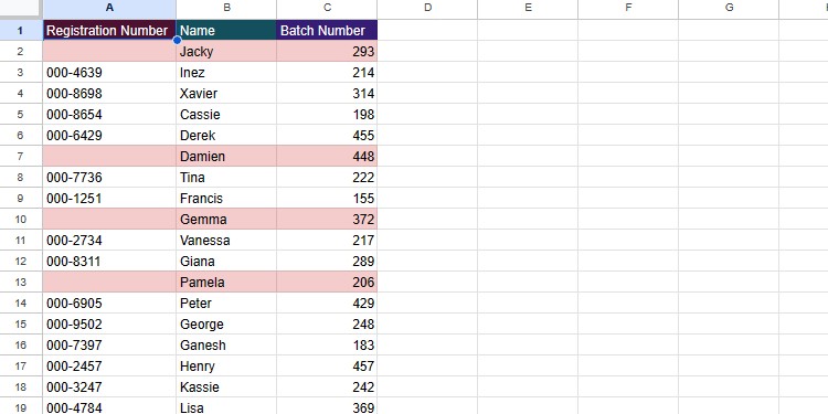
We need to import the names of students who have a registration number using the IMPORTRANGE and QUERY function.
On our destination sheet, here is how we construct a formula nesting QUERY to match this criterion:
=QUERY(IMPORTRANGE("https://docs.google.com/spreadsheets/d/1yMCNRqp-hf8c0zuJjXg55RuZR2BYKL2L3BlseTJ1Q2Q/edit#gid=888095793","Sheet3!A1:B41"),"select Col2 where Col1 is not null",0)