When you reference any cell from a pivot table, instead of the values, you will get a GETPIVOTDATA formula. This might confuse you if you are new to Excel or pivot table in general.
So what is GETPIVOTDATA, and why is it so important to use it on a PivotTable?
The GETPIVOTDATA function is classified under the lookup and reference functions and is used to look up values in a PivotTable.
You may be thinking, “Aren’t there other functions like VLOOKUP to get values from PivotTables?” Well, no. GETPIVOTDATA is a dedicated function to get values from a PivotTable. In this article, we will be giving you a general overview of the GETPIVOTDATA and why you should be using it in PivotTables in Excel.
What is GETPIVOTDATA in Excel?
GETPIVOTDATA is a fairly old function in Excel. It uses the date field and PivotTable names to extract value from a PivotTable.
What makes GETPIVOTDATA so special is that it does not depend on the cell location to extract values. This means, even if you hide the referenced cell from the PivotTable, the values remain intact. This is quite the opposite of VLOOKUP, which triggers the #N/A error when you hide the source range.
Arguments used in GETPIVOTDATA in Excel
Let’s dive deeper into what GETPIVOTDATA is by analyzing the arguments it uses. Here’s how GETPIVOTDATA is used when constructing a formula in Excel:
=GETPIVOTDATA(data_field,pivot_table,[field1_item1],[field2_item2],[field3_item3]...)| Argument | Data Type | Description |
| data_field | Text | The field you wish to extract your value from. This is generally the column or row header. |
| pivot_table | Cell Reference | The row label of your PivotTable. This can be any reference under the label. |
| [field1,item1] | Text | The name of the reference field and its item. |
Let’s select a random value in your PivotTable and analyze it to see how GETPIVOTDATA works in Excel.
I selected a field value in cell I8. Instead of getting =I8 in the formula bar, I received the =GETPIVOTDATA("Cost",$H$1,"Item Purchased","Refrigerator") formula. This formula is commanding Excel to retrieve the value in the data_field “Cost”, from the PivotTable in cell $H$1.
As it is a specific value, this formula has also specified the field name, Items Purchased, and Refrigerator as a reference. Using these references, the formula extracts data from the data field, Cost.
How to Use GETPIVOTDATA in Excel?
We have arranged a list of examples to help you understand the application of GETPIVOTDATA in Excel.
Example 1: Get the PivotTable Summary Using GETPIVOTDATA
When you create a PivotTable, it automatically creates a summary of your values. In this PivotTable, the summary of field, “Cost” is next to the label, “Grand Total”. As this is a smaller PivotTable, analyzing this data is easier, however, you would have to use GETPIVOTDATA in case of a larger PivotTable.
Here’s how I constructed my formula using the GETPIVOTDATA function to get the summary of my values:
=GETPIVOTDATA("Cost",$H$1)Example 2: Look Up a Value Using GETPIVOTDATA
This is probably the most used application of the GETPIVOTDATA function. When you extract value using the GETPIVOTDATA, even when you change the field and its values, the value remains unfazed. This way, you can analyze other data while still viewing data from other fields.
Let’s use GETPIVOTDATA to look up the “Sum of Cost” value of the item, “Stove”. This is how I created the formula:
=GETPIVOTDATA("Cost",$H$1,"Item Purchased","Stove")Example 3: Look Up Values using Dates in GETPIVOTDATA
You can refer to months from serial numbers 1-12 in the GETPIVOTDATA formula. Similarly, quarters are grouped from 1-4. Instead of entering the month and quarter names, you have to enter the serial numbers to look up a value.
In this PivotTable, we have arranged each Item Purchased and their Cost values under Jan and Feb. If you look closer, the item, Stove was purchased in both Jan and Feb. Let’s create a lookup formula using GETPIVOTDATA to extract the total cost of purchasing Stove in the month of Jan.
=GETPIVOTDATA("Cost",$A$21,"Item Purchased","Stove","Months (Date)",1)Here, the field we’re looking for data from is Cost. Therefore, that will be our argument for data_field. As our PivotTable start from cell $A$21, that will be our next reference. The item we’re looking for the cost for is Stove, which is in the Item Purchased field. Therefore, they will be our next arguments.
Moving on, we’re looking for the cost of the Stove for the month of January. In our PivotTable, months are grouped under the Months(Date) field. As Jan is denoted by the serial number 1, these values will be our second field and item respectively.
Errors in GETPIVOTDATA
When learning a new function, we oftentimes stumble over a few errors. Here are some of the common errors you may encounter when learning to use GETPIVOTDATA correctly in Excel:
#REF! Error
If you keep getting the #REF! error, even when you have correctly typed in your formula, it is because your field item isn’t currently visible on the sheet. Try bringing the data back on the spreadsheet and see if it resolves your issue.
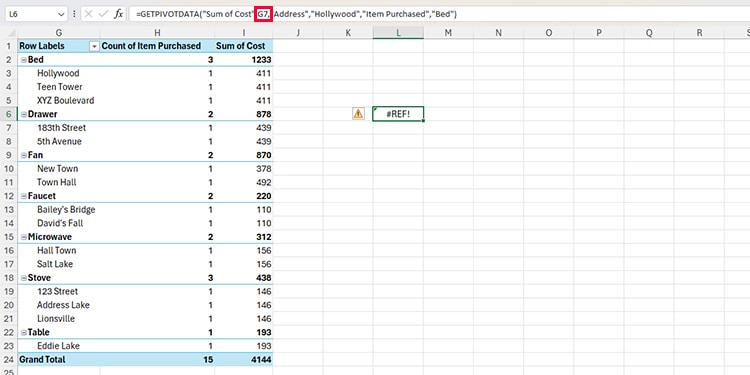
If you’re still facing issues, check your formula and the cells you’ve referenced again.
#NAME? Error
You will mostly encounter the #NAME? error in Excel if you’ve mistyped the name of your function. This is more of a common occurrence when learning a new function and it definitely doesn’t help that GETPIVOTDATA is a long name for a function.
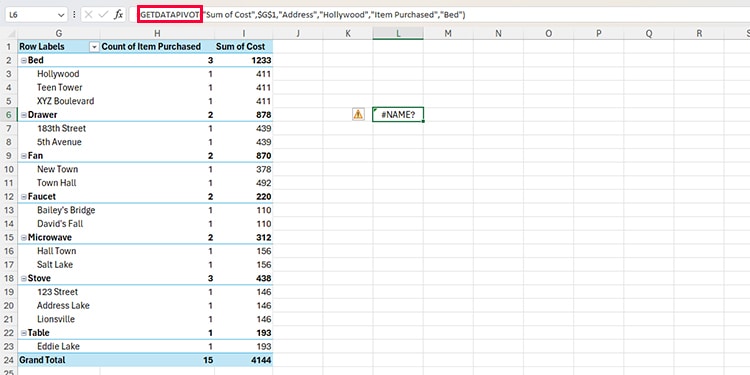
To avoid the #NAME? error, use the Insert Function tool when creating or using a formula in Excel. You can look for functions through their category or even their description.
Incorrect Result
When learning a new function, you may sometimes end up with an incorrect result. Don’t worry, mistakes are a part of the learning process.
If your formula returns an incorrect result, select the cell and check the formula in the formula bar. Make sure you’re referencing the correct data_field. You can check the data_field from the PivotTable’s Field List.
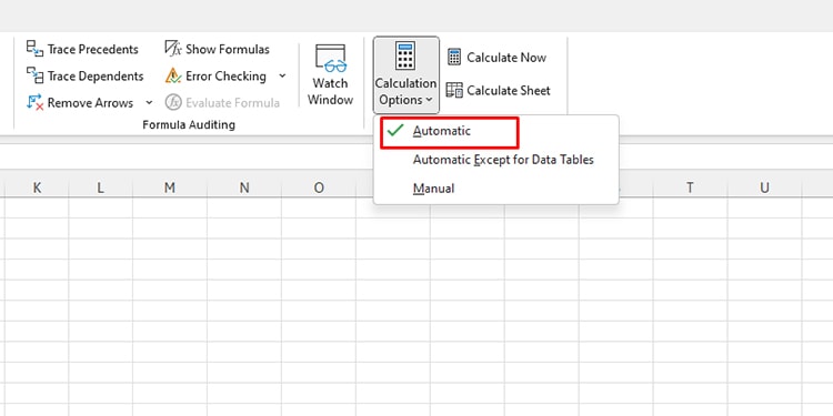
Formula Not Updating Dynamically
You could’ve enabled manual calculation in your Excel program if your formulas aren’t updating dynamically. You can use F9 on your keyboard to refresh your spreadsheet or head on to the Formulas tab to change your calculation to automatic.
- Go to the Formulas tab.
- Select Calculation Options from the Calculation section.
- Choose Automatic.
How to Avoid Errors using the GETPIVOTDATA
Sometimes, you know you’re bound to get an error using the GETPIVOTDATA. Especially when the data you’re requesting to lookup is currently unavailable in your sheet. Errors are never a good look in the spreadsheet. Therefore, you can nest the GETPIVOTDATA function inside the IFERROR function to avoid displaying any errors.
Arguments Used in IFERROR
Here’s how IFERROR is written in a formula:
=IFERROR(value, value_iferror)Nest GETPIVOTDATA inside IFERROR
This is how you can next your GETPIVOTDATA function inside the IFERROR function to avoid displaying Excel errors:
=IFERROR(GETPIVOTDATA(data_field,pivot_data,[field_1,item_1],[field_2,item_2],...),0)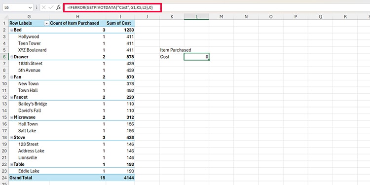
This formula returns 0 instead of any Excel error.