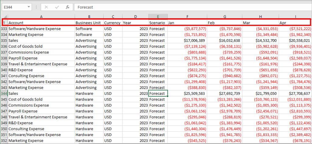
If you’re working with giant spreadsheets, Rows and Columns can go pretty far. In such situations, you’d have to keep scrolling back and forth to view any information.
Assuming you need to look up the data of 1050 Row. By the time you reach the cell, you’d lose track of headings which makes data reading very complex.
To overcome this, Excel’s often overlooked feature, Freeze Panes can be very useful. This option provides the ability to lock certain rows and columns of a worksheet. Thus, you can still keep them visible while scrolling.
Using Shortcut Key
Firstly, we have keyboard shortcuts to freeze panes of your worksheet. These shortcut keys can make your work faster and more efficient. All you have to do is select a cell and press down the following keys together.
Freeze Top Row: ALT + W + F + R
Freeze First Column: ALT + W + F + C
Freeze Panes: ALT + W + F + F
To explore more Excel shortcuts, you can check out our other article on 200+ Excel Keyboard Shortcut.
Using Freeze Panes
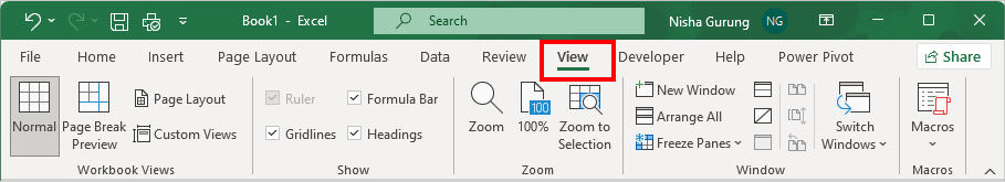
Excel has a default Freeze Panes menu in the View Tab. If you cannot keep tabs on keyboard shortcuts, use this method.
Freeze Top Row
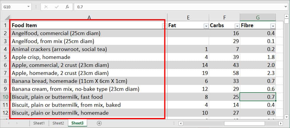
In most cases, the top row of your worksheet consists of Heading. So, while you are scrolling through huge datasets, you would want to lock only the top row to keep up with the data heading. For example, in Records like the given picture.
For this, while freezing panes, you can pick an option to Freeze Top Row. Excel will lock Row 1 by default. However, if you have hidden Row 1 and Row 2, Excel will identify Row 3 as the first Row and freeze it instead.
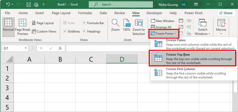
Now, to lock top row,
- Open your worksheet and go to View Tab.
- From the Window menu, choose Freeze Panes > Freeze Top Row.
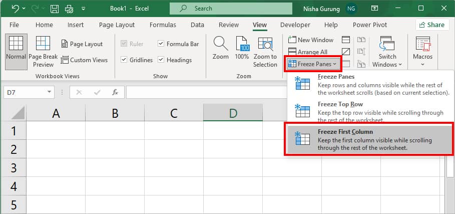
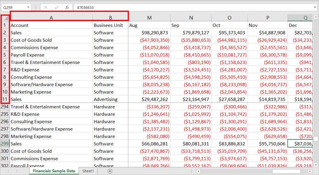
Freeze First Column
Sometimes, the first column of your document contains significant information like in the given picture. In such cases, Freeze First Column to only keep them visible while you’re navigating through other Columns.
Here, Excel will lock the first column of A1 by default.
- Select the Area of your worksheet you want to freeze.
- Click on View Tab.

- Click Freeze Panes > Freeze First Column.
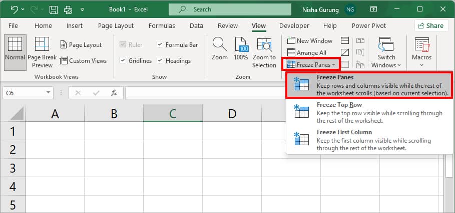
Freeze Panes
The above-mentioned options will freeze only the top row and column of your worksheet. However, there can be times when you want to lock both Row and Column. In such case, pick the Freeze Panes option.
One of the most important things you must note while freezing panes is your Active cell. Excel locks all the above rows and left columns of the current selection. For example, C12 is an active cell in the worksheet. The Freeze Pane option will lock all the Rows till C11 including Columns A and B. Very thin line will appear in the locked area.
Now, to freeze panes,
- On your worksheet, select the Cell.
- Navigate to View Tab.

- On Window section, click Freeze Panes > Freeze Panes.
Related Questions
How to Unfreeze Panes?
To Unfreeze Panes, navigate to the same Freeze Panes menu in the View Tab like you did earlier. Then, click on Freeze Panes > Unfreeze Panes. This menu will unlock all locked rows and columns.