How to Count Significant Figures in Excel

When you have decimal numbers in Excel, you might not know whether you’re overrepresenting or excluding the important figures during the calculation.

To have the precise number in calculations, you could count only the significant figures. It is the total number of important digits you count in a numerical value from the left side.

Here, you must consider the value zero and the decimal when counting them. So, before we dive into the steps directly, let’s quickly recap the rule for Significant Figures.

• Leading Zeros: It is never significant. Suppose, you have a 0.00703 number. Here, only 3 numbers 703 is a significant figure.
• Between Zeros: The Zero that lies in between non-zero digits is counted. In number 705.001, the significant figure is 6. 
• Trailing Zeros: It is not counted when there are no decimal digits. For example, in 700, there’s only 1 Significant figure 7.
  But, if there’s a decimal or leading zeros at the front, it is counted. Example: 10.0 has 3 significant figures. Similarly, 0.005000 has 4 figures which is 5000. 

Now, let’s count these Significant Figures such that you have the exact required numbers in Excel. 

Count Significant Figures Using Formula

To count, we will use several functions nested together. Depending on how your number is stored in Excel, use Example 1 or 2. 

Example 1: Numbers Stored as Number

Suppose, I have lists of numbers from cell A3 to A9. Let’s count the Significant Figures in the Column B.

For that, I used this formula and used the + cursor to copy it down to the remaining columns.

=IF(A3="","",IF(ABS(A3)=0,0,LEN((ABS(A3)/10^LEN(ABS(A3)))*10^(LEN(ABS(A3)/10^LEN(ABS(A3)))-LEN(INT(ABS(A3)/10^LEN(ABS(A3))))-1)))+LEN(A3)-LEN(ABS(A3))-IF(LEFT(A3,1)="-",1,0)+IF(OR(LEFT(A3,1)=".",LEFT(A3,2)="-."),1,0))+IF(AND(NOT(ISERROR(FIND(".",A3))), ISERROR(FIND(".",ABS(A3)))),-1,0)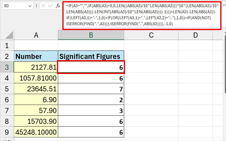

Since the formula is long, you might make mistakes when typing it one by one. Instead, just copy-paste the formula on your sheet and replace the A3 cell reference.

As per the Significant Figure rule we’ve mentioned above, the formula counted only important digits. It returned 6 for a 2127.81 number. 

Example 2: Numbers Stored as Text

Let’s say, here I have numbers in text format. We will find out the Significant Figures without changing the cell format.

For that, I used the formula mentioned in the box. Use the copy-paste command to insert the formula in your sheet and change the cell reference.

=LEN(MID(SUBSTITUTE(SUBSTITUTE(B3,".",""),",",""),AGGREGATE(15,6,ROW($XFD$1:INDEX(XFD:XFD,LEN(SUBSTITUTE(SUBSTITUTE( B3,".",""),",",""))))/(MID(SUBSTITUTE(SUBSTITUTE(B3,".",""),",",""),ROW($XFD$1:INDEX(XFD:XFD,LEN(SUBSTITUTE(SUBSTITUTE(B3,".",""),",","")))),1)<>"0"),1),99))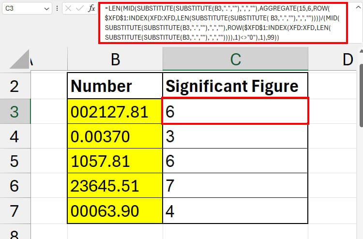

In the cell C3 for 002127.81 number, I got 6 significant figures. Once you get the result, drag down the Auto-Fill handle to update the entire column. 

Count Significant Figures Using VBA

For users who need to use the formula regularly to count significant numbers, I have constructed a VBA to insert a custom function. It’s the best way to avoid redundant tasks and save your time. 

The code will add a function named SignificantFigure. In the code, I have set two function arguments which are number and case.

To create this function, follow the given steps. Check and load the Developer Tab before you start.

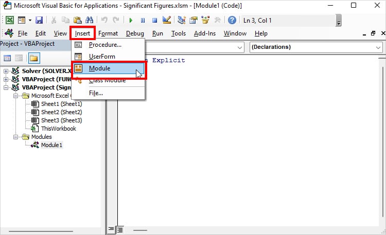
1. First, open the VBA window in your worksheet using the Alt + F11 shortcut keys.
2. Click Insert > Module.
   
3. Copy and Paste Code.
   

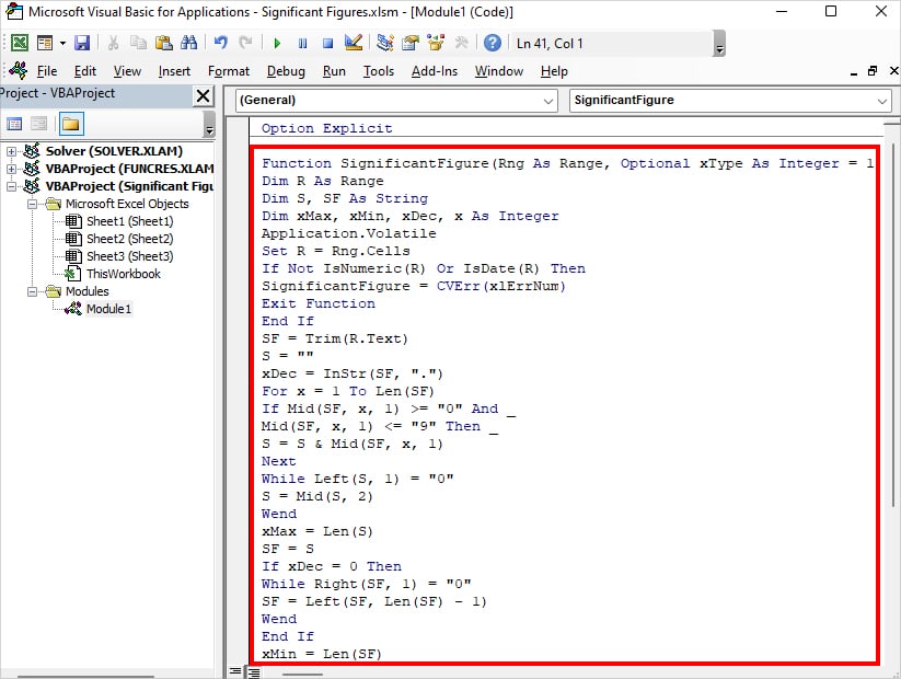
Option Explicit
Function SignificantFigure(Rng As Range, Optional xType As Integer = 1)
Dim R As Range
Dim S, SF As String
Dim xMax, xMin, xDec, x As Integer
Application.Volatile
Set R = Rng.Cells
If Not IsNumeric(R) Or IsDate(R) Then
SignificantFigure = CVErr(xlErrNum)
Exit Function
End If
SF = Trim(R.Text)
S = ""
xDec = InStr(SF, ".")
For x = 1 To Len(SF)
If Mid(SF, x, 1) >= "0" And _
Mid(SF, x, 1) <= "9" Then _
S = S & Mid(SF, x, 1)
Next
While Left(S, 1) = "0"
S = Mid(S, 2)
Wend
xMax = Len(S)
SF = S
If xDec = 0 Then
While Right(SF, 1) = "0"
SF = Left(SF, Len(SF) - 1)
Wend
End If
xMin = Len(SF)
Select Case xType
Case 1
SignificantFigure = xMin
Case 2
SignificantFigure = xMax
Case Else
SignificantFigure = CVErr(xlErrNum)
End Select
End Function

4. Press Save. Excel will send you a warning saying there’s a Macro. You can check out our article to learn how to save Macro containing Workbook.

Now, use the function. Here, I entered =SignificantFigure(C2, 1) in cell D2. The formula returned 6.

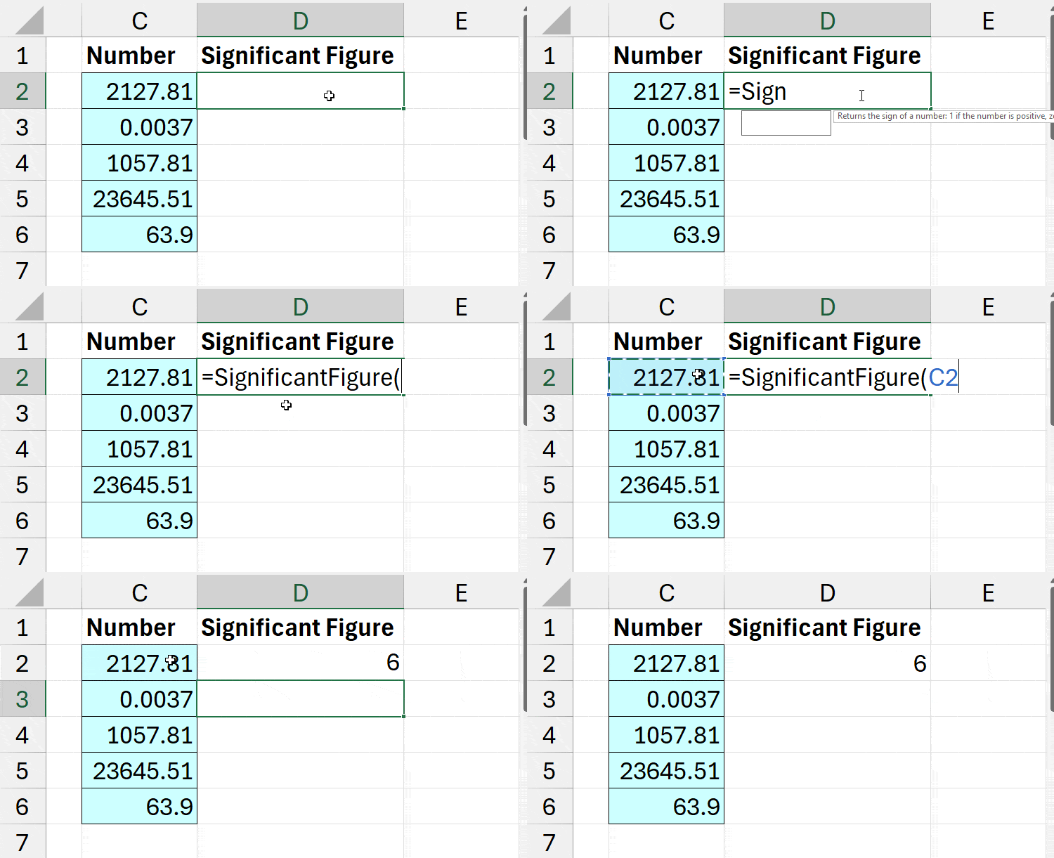
To apply the formula, drag down the Auto Fill Handle.