How to Make Excel Drop Down List with Color (Step-by-Step Guide)

While the dropdown lists speed up the data entry process, they still look like normal cells without color formatting.

Although you could manually color each cell, their formatting remains the same even if the user selects a different value from the dropdown list.

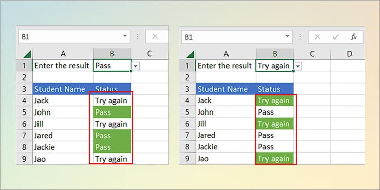
To avoid it, you need to incorporate one or more conditional formatting rule (s) into your dropdown lists. Then, the color will automatically change based on the active value.

In this article, we go through each step to create a dropdown list and explore various conditional formatting options you can apply to them.

Step 1: Create a Dropdown List

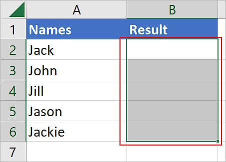
Select the cell (s) where you want to include the dropdown list.
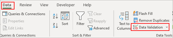
Go to the Data tab.
Then, click Data Validation inside the Data Tools section.
Next, choose the List option under Allow.
Now, click the Up arrow under the Source section and select the cells which contain the dropdown values.
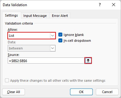
Click OK.

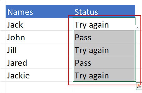
Step 2: Select the Cell(s) Containing Dropdown Lists

Once you create dropdown lists, select them to apply conditional formatting.

Step 3: Apply Conditional Formatting Rules

After you select the dropdown lists, it’s time to color them with various conditional formatting rules. For that,

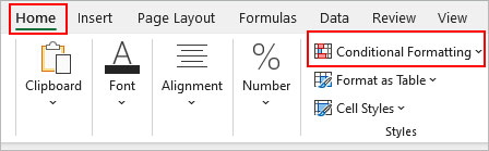
Go to the Home tab
Select Conditional Formatting > Highlight Cells Rules.
Now, choose the preferred conditional formatting rule(s) as mentioned below.
- Highlight cell rules: Using this rule, you can color the cells with dropdown options containing values greater than, less than, between, and equal to a specified number. For instance, color all the cells with dropdown values greater than 30 with green.
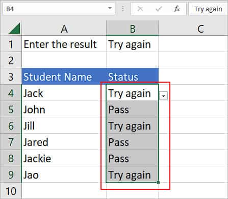
- Text that Contains: This rule lets you select all the cells with dropdown values containing a particular text. However, the text doesn’t need an exact match to apply the rule. Meaning, if you create a rule that contains the text “try,” it can select the text “try again” also.
- A Date Occurring: This option colors all the dropdown cells within a date range such as yesterday, previous month, next month, etc. However, note that you cannot choose a custom date.
- Duplicate Values: This rule allows you to color all the cells with similar values actively selected on the dropdown list. For instance, you can select all the cells with the same value “Jackie” under the Assigned To column.
- Data Bars: Data bars are quite useful to visually represent your data with colors. Among the cells where you have applied the conditional formatting, cells with the biggest numbers are represented with big data bars. And likewise for the smaller numbers.

Step 4: Apply a Custom Conditional Formatting Rule (Optional)

If the above options don’t suit your particular situation, you can highlight your cells with dropdown values using a custom conditional formatting rule.

Using it, you can cover all the dropdown list values with almost any type of data validation. Also, you can combine several functions and create a powerful formula to highlight cells based on specific dropdown values.

To use it,

Select the cell (s) where you need to apply the color based on the dropdown value.
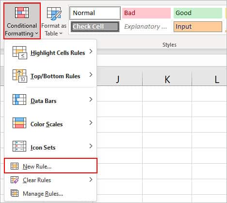
Under the Home tab, select Conditional Formatting > New Rule.
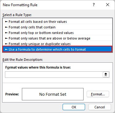
On the New Formatting Rule window, select the Use a formula to determine which cells to format option.
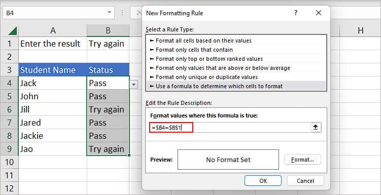
Under the Format values where this formula is true section, enter your custom formula. Here, we are trying to color those cells which contain the same value selected in the dropdown value.
Then, click the Format button below.
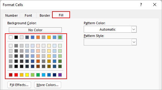
Choose a preferred background color under the Fill tab. To check other colors, click More colors.
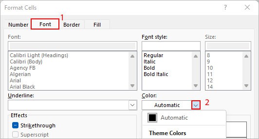
Additionally, select the Font tab and choose your preferred font color under the Color section. You can also manage other font settings according to your preferences.
When done, click OK.
In our example, the final output looks like this. As you can notice, the cells are highlighted with the green color based on the active dropdown list value next to Enter the result.