How to Name and Use Dynamic Named Range in Excel

Once you name a cell range, you can reference it anytime when writing formulas. However, it only covers those specific cell references and isn’t dynamic.  

Meaning, any additional data (cell value or a whole record) you insert at the start/end of the named cell range isn’t included. Thus, you need to manually update the cell reference of the named range to include them again.

So, a better approach is to use the dynamic named ranges which include the new entries automatically, and update the named range itself. 

Using Excel Table

A much more convenient and easier way to use a dynamic name range is to convert the named range into a table. Using it, you can easily insert additional column/row entries without having to re-edit the named range.

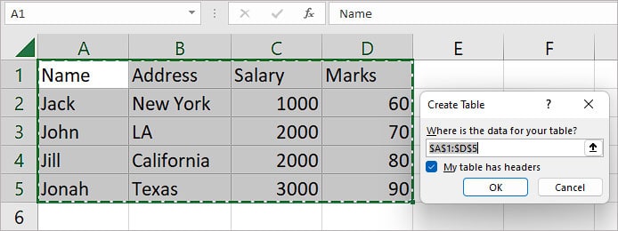
1. Select the table. If you haven’t converted the required cell range into a table, press Ctrl + T. Then, enable the My table has headers checkbox to include the header (column name). 
   
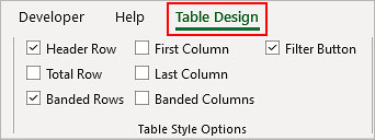
2. By default, Excel names each table sequentially such as Table1, Table2, etc. To make the table name more meaningful, select the Table Design tab.
   
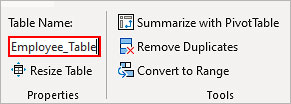
3. Then, replace the default name with another appropriate table name such as “Employee_Table”. You can find the option in the top-left corner.
   
4. Now, as you add a new entry (Row 6 in this case) across the adjacent row or column of the table, it automatically adjusts to include them as well without manually changing the cell reference.
   

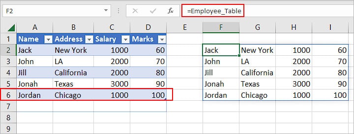
On top of using the whole table as a dynamic named range, each column inside can be separately used as a named range. 

The good part is, you don’t even need to name the columns manually. Each cell range in a table column takes up its header name as the named range.

Also, when referencing a table column inside a formula, Excel uses column names such as Address instead of the cell reference like A2:A10. Such references are specifically called structured references.

For example:
=SUM(Employee_Table[Salary])

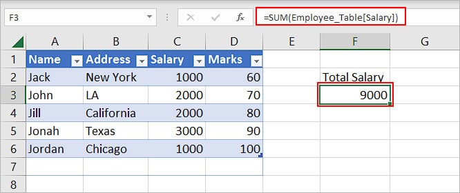
Here, Employee_Table is the table name and Salary is one of the column names inside that particular table. As a whole, the above formula calculates the total salary by adding cell values inside the Salary column of the Employee_Table.

To specify a column in a table, Excel uses a column specifier, which includes the column name wrapped in square brackets just like [Salary] in the above example.

Furthermore, you can use several special item specifiers like the following.

• #All: returns the whole table data including any headers and the totals row. 
• #Data: returns the table data part only, excluding the table header
• #Headers: returns only the header part of the table

In combination with the table name and column specifier, you can use the special specifiers to extract specific table data. And, they are separated with a comma.

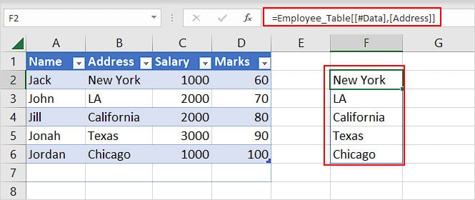
For instance, in the image below, the formula =Employee_Table[[#Data],[Address]]returns all the data part of the Address column inside the Employee_Table table.

Using the OFFSET Function

Another way you can use a dynamic named range is to convert the existing named range into a dynamic one. Here, we use the OFFSET function along with the COUNTA function.

However, note that the dynamic named range created using this method won’t appear in the name box, so you have to look it up in the name manager or remember the name. Also, you need to create a custom OFFSET formula for each named range and adjust cell references according to your data.

So, you can consider this method if you don’t want to be converting your data into tables and avoid any sort of compatibility issues when using tables in another Excel version.

1. Select the Formulas tab and click Name Manager.
   
2. Choose the named range you want to convert into a dynamic named range and click Edit.
   
3. Next to the Refers to field, use the following formula according to your cell reference. When you select the cells, Excel automatically inserts the Sheet so you won’t have to type it manually.
   =OFFSET(First_cell, 0, 0, COUNTA(Column)-1, 1)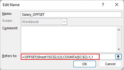
   
4. Click OK.

To understand the formula better, let’s take a look at an example.

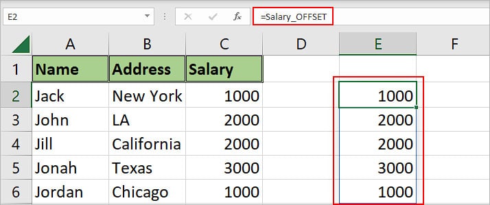
In the above image,  we have used the =OFFSET($C$2,0,0,COUNTA($C:$C)-1,1 formula.

Where,

• $C$2 is the cell reference of the first entry of the Salary column.
• $C:$C refers to the cell reference of entire cells in column C.
• COUNTA($C:$C) searches for all the non-blank cells across the entire column C and finds 6 of them including the header. But, since we don’t want the header we subtract it. That’s why the formula is COUNTA($C:$C)-1 in the above example.

Using the INDEX Function

You can also use the INDEX function to use a dynamic named range. However, it can be a little complex if you are just an Excel beginner and don’t know much about various Excel functions and formulas.

Also, you have to re-adjust the formula according to your data for each named range you want to convert to a dynamic one. And, similar to the OFFSET method, you can use this method by replacing the named range’s reference with its formula.

For instance, 
=$A$2:INDEX($A:$A,COUNTA($A:$A))

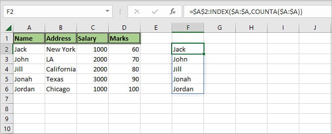
Here,

• $A:$A refers to all the cells inside column A.
• COUNTA returns the number of non-blank columns. So since we are starting from $A$2 (Jack), we get 6.
• INDEX($A:$A,6) searches the whole column and returns row number 6 (Jordan), whose cell address is $A$6. 

So, the formula becomes=$A$2:INDEX($A:$A,6))and evaluates to =$A$2: $A$6. Which means, the new entry Jordan in row 6 is also included by our named range.