How to Create Dependent Drop down List Excel

The dropdown lists make the data entry process much easier by letting users choose from the pre-defined options.  This eliminates the need to enter the input manually and avoids any errors while typing them.

However, when you start using multiple dropdown lists, the list of options may get too long if you treat each of them as an independent list. To avoid it, there’s a better alternative, which is to use dependent dropdown lists.

By creating such lists, you can display specific options on one drop-down list based on what value the user chose on another drop-down list. Also, you can prevent users from selecting an invalid combination of dropdown options and only display the relevant options.

Using the INDIRECT Function

The INDIRECT function can be specifically used to create dependent drop-down lists in Excel.

Syntax:=INDIRECT(ref_text)

Here, the function takes ref_text as input and tells Excel to look at the exact text which refers to a cell range.

Step 1: Create the First Dropdown List

You need to have at least two dropdown lists to use a dependent drop-down list. So, create the dropdown lists according to your requirements using Data validation.

Step 2: Create Named Ranges

Now, assign a named range for each option you want to use in the second dropdown list depending on the values selected in the first dropdown.

However, make sure the named ranges match their name exactly with the first dropdown list options. That is because the INDIRECT function is case-sensitive. Meaning, it interprets Models and models as different things.

For this, 

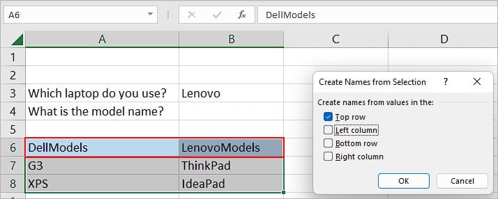
1. Select all the dropdown list options and preferably use the first drop-down options as headers with dependent drop-down options under them. Here, the first dropdown list contains {Dell, Lenovo} and the dependent drop-down options {G3, XPS, ThinkPad and IdeaPad) are below them.
   
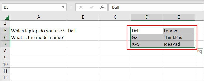
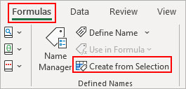
2. Now, click Create from Selection under the Formulas tab.
   
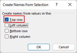
3. Enable the Top row checkbox. Here, it’s at the top but choose other options depending on where your header is.
   

Step 3: Use the INDIRECT Function

1. Now, select the cell (s) where you want to insert the second dropdown (dependent dropdown).
   
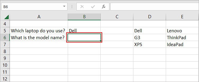
2. Then, select Data Validation under the Data tab.
   
3. Choose List under Allow. Also, make sure the In-cell dropdown checkbox is enabled.
4. Under the Source field, type =INDIRECT() and enter the cell reference of your main dropdown.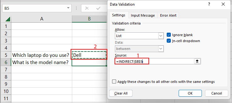
   
5. Click OK.

Using the IF Function

Another way you can create dependent dropdown lists is by using the IF function. It basically checks if a condition is true or false and carries out the corresponding task.

Syntax:=IF(condition, task if true, task if false)

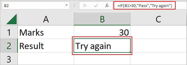
For instance,
=IF(B1>=30,”Pass”,”Try again”)

In the above example, we are telling Excel to check if the cell value of B1 is greater than 30. Then, it returns “Pass” whenever the condition is true and “Try again” whenever false.

Moving on to creating a dependent drop-down list, you follow similar steps as in the above INDIRECT method. 

Step 1: Create the First Dropdown List

Step 2: Create Named Ranges

Unlike the INDIRECT function, this method works even if the named ranges for the header of the second dropdown list options don’t match the first dropdown list options. You can create the named ranges using the Create from selection option as mentioned in the above method.

Step 3: Use the IF function

1. Select the cell (s) where you want to insert the second dropdown list.
2. Then, click Data Validation under the Data tab.
3. Under the Source field, type =IF($B$3="Dell", DellModels, LenovoModels). Here, depending on whether the B3 cell contains Dell or Lenovo, we are telling Excel to display their respective model options.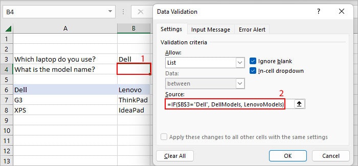
   
4. Click OK.

How to Create a Dynamic Dependent Drop-down List?

If you later decide to add more options to your dropdown list, the named range won’t expand to include them automatically. So, it’s better to use a dynamic named range while creating the dropdown list.

One such way is to use tables. In addition to the list being dynamic, the structural references make it even easier to reference a cell range.

Let’s look at an example.

1. Create the first dropdown.
2. Make separate columns for each of its options and place all the dependent dropdown options under it. Then, select all and convert them into a table.
   
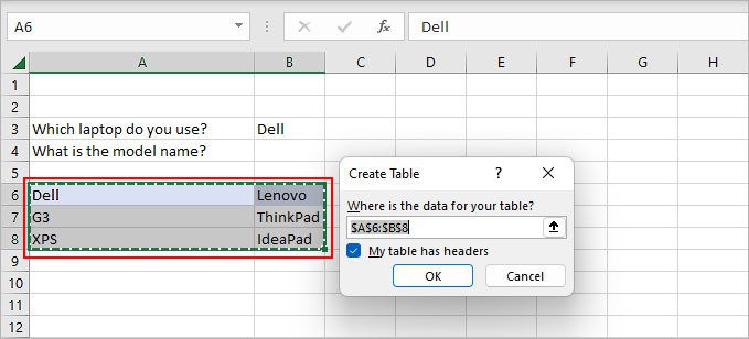
3. Then, select the whole table and assign named ranges for each of its columns using the header names. You can do so using Create from Selection. 
   
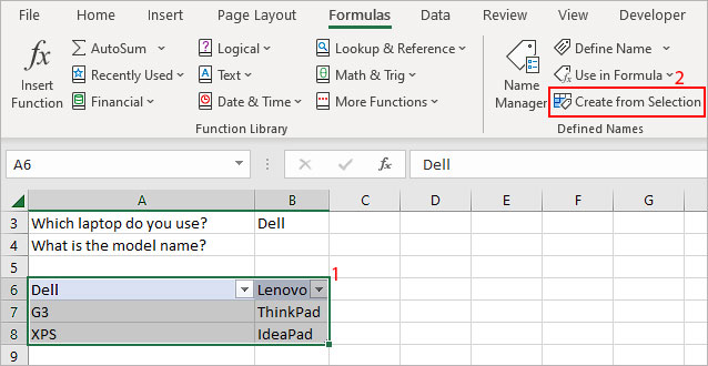
4. Now, while creating the dependent dropdown list, you can use the INDIRECT function similar to the above.

After you create the dynamic dropdown list, you can now notice that when we added new model entries, the dependent dropdown included it automatically.

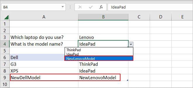
How to Reset a Dependent Dropdown List?

One major issue you can face while using a dependent dropdown list is that dropdowns do not reset. Meaning, if you choose an option in the dependent dropdown and again change the first dropdown list value, the second one will still have the same value.

For instance,

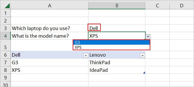
In the above image, since we chose Dell in the first dropdown list, the dependent dropdown list only displayed Dell models. 

However, once we choose a model, we can still change the first dropdown value. But, the second dropdown value is still active as we can see in the image below. As a result, it resulted in an incorrect dropdown option combination.

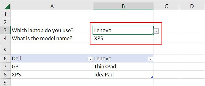
What we want is, whenever the user once selects the options from both dropdown lists, we want the dependent list to reset automatically.

For this, we can use the VBA as follows.

1. Right-click on the worksheet containing the dependent drop-down list and select View Code.
   
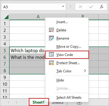
2. On the main window, select Worksheet.
3. Then, enter the VBA code with proper indentation.
   
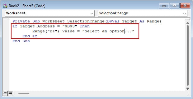
4. Close the VBA window and save the worksheet. Click Yes on the next prompt.

Note: In the above code, $B$3 is the cell reference of the first dropdown list and B4 refers to the dependent dropdown list. Replace the cell reference accordingly for the VBA code to work.