While Excel has several tools for removing duplicate values from a cell range, you may occasionally need to count them instead.
This is particularly useful if you want to identify your most frequent customer or pinpoint which products are selling the most. In such cases, knowing the frequency of duplicates can help you make strategic plans and increase your sales.
In this article, we explain how you can check for the total number of duplicates in a single column. Also, you can find the frequency of duplicate records/rows too.
Before you begin, save a copy of the original data so that you can revert to it in case you get a different result than expected. And, it's better to convert your data into a table (Ctrl + T) as it automatically counts any new duplicate entry you add later.
Case 1: Total Number of Duplicates across Rows or Columns
To find the total number of duplicate records in single/multiple columns, you can consider the Remove Duplicates option or use the COUNTIF function.
But, if you are also looking for the number of duplicates for each item in the column or count duplicate records in the dataset, continue reading.
Using the Remove Duplicates Method
- Open the worksheet that contains the data and select a cell on your dataset.
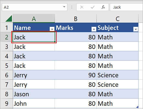
- Click the Remove Duplicates icon inside the Data Tools section. You can find it under the Data tab.

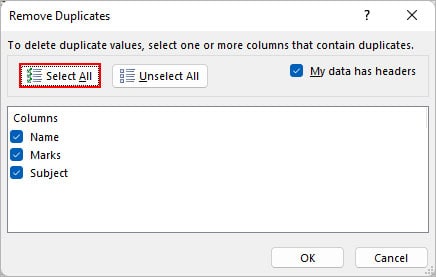
- On the Remove Duplicates prompt, click Select All to check the total number of duplicate rows/records.
- To check for duplicates in a single column, click Unselect All and only enable its checkbox. Here, we selected the Name column to count the total number of duplicate names in it.
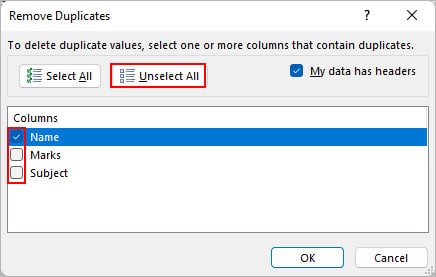
- Also, enable the My data has headers checkbox.
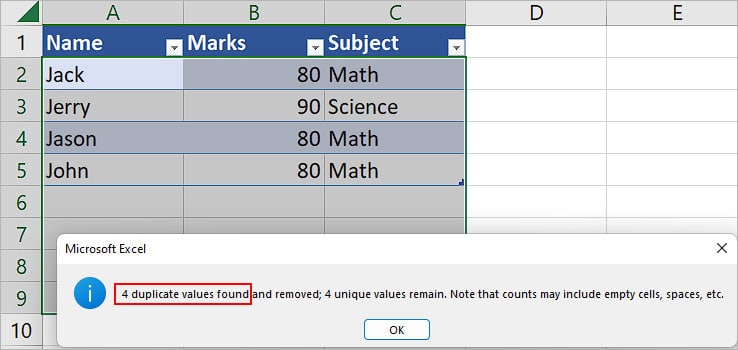
- On the next prompt, check the total number of duplicate records. Here, the record
{Jack,80,Math}repeated four times and had three duplicates.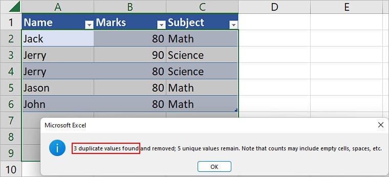
- Similarly, while checking for duplicates in the Names column, the name Jack had three duplicates and Jerry had one, resulting in a total of 4 duplicate values.
Using the COUNTIF Function
To directly find the total number of duplicates inside a column, you can use the COUNTIF function in combination with the UNIQUE function.
Syntax: =COUNTIF(cell range,criteria)
Where,
- Cell range: cell reference of the cells inside the column
- Criteria: cell reference of the item to check for duplicates inside the column
Similarly, the syntax for the UNIQUE function is =UNIQUE(range)
Where,
- Range: cell range from which you want to extract unique items only
Now, we can use the following formula as follows.
=COUNTA(cell range)-COUNTA(UNIQUE(cell range))
Let’s take a look at an example to better understand the use of the above formula.
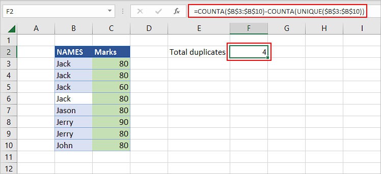
Here,
COUNTA returns the total number of non-empty cells. But, note that it will still include the cells that contain spaces while counting.
The UNIQUE function returns the cells containing only the unique values.
So, we can evaluate the above formula as follows.
COUNTA($B$3:$B$10)-COUNTA(UNIQUE($B$3:$B$10))
Where,
COUNTA($B$3:$B$10) returns 8.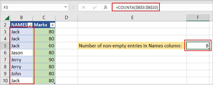
UNIQUE($B$3:$B$10) returns a list of unique names.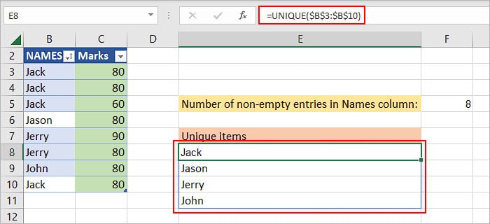
Thus, the COUNTA(UNIQUE($B$3:$B$10)) function returns 4 as there are four unique names. So, the whole formula COUNTA($B$3:$B$10)-COUNTA(UNIQUE($B$3:$B$10)) evaluates to 8-4, which equals 4. 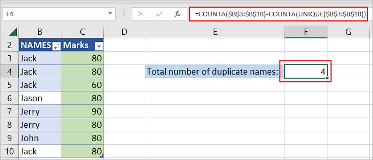
Case 2: Find the Number of Duplicates in a Single Column
Using the COUNTIF Function
Using the COUNTIF function, you can calculate the total number of occurrences of an item inside a column.
For instance, =COUNTIF(A: A, A1) checks for every occurrence of the A1 cell value in the entire column A.
After finding the occurrence of each item, you can subtract 1 from them to calculate the total number of duplicates for each item.
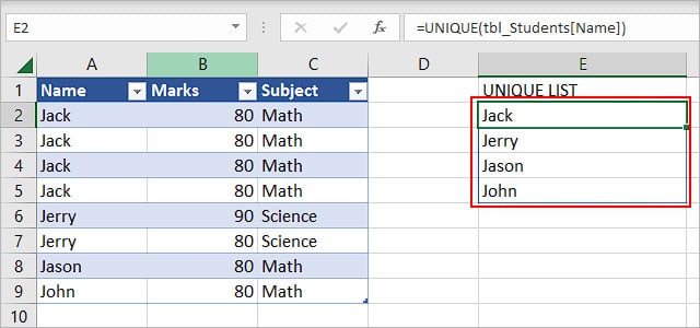
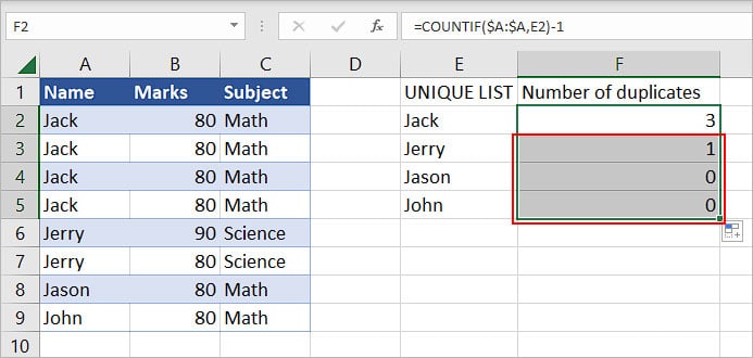
- Create a helper column and give it an appropriate name such as “Unique List”. Then, extract the unique items there. You can use the UNIQUE function as mentioned above. Since we converted our data into a table, we used the structured reference here. But, you can just enter the name column’s cell range (A2:A9) if it’s easier for you.
- Create another helper column to display the frequency of each duplicate item. Here it’s called “Number of duplicates”.
- Use the COUNTIF function to search for duplicates of one item. Here, in the formula,
=COUNTIF(A: A, E2)-1, we are counting the number of times the E2 cell value (Jack in this case), has appeared across the whole column A, except for the first occurrence.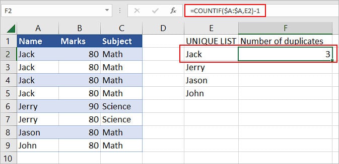
- Then, use the drag handle to find the total number of duplicates for other items in the list.
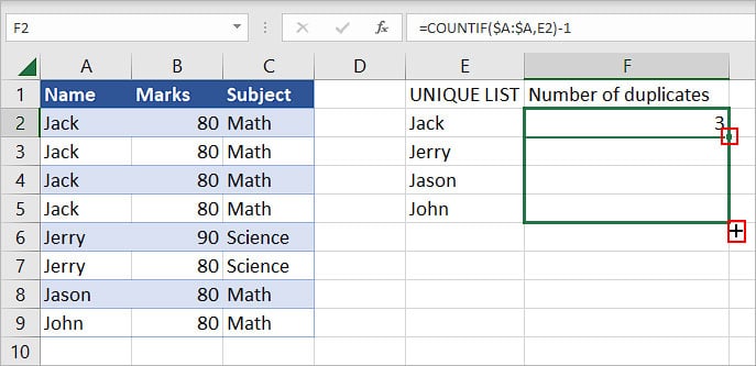
- After using the drag handle, the final result is as follows.
Case 3: Count Duplicate Records/Rows
Counting duplicate records requires some additional steps. Here, you merge all the columns into one after which you can calculate the number of duplicates similar to how we calculated for a single column.
Step 1: Merge Columns
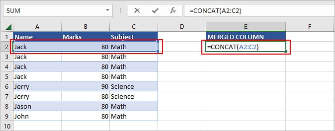
First, create a helper column that will contain all the merged columns. To merge the columns, you can use the CONCAT function.
Syntax:=CONCAT(cells you want to concatenate)
To concatenate cell values of multiple columns, type =CONCAT(, and select a row/record. Then, enclose the round bracket to complete the formula and press Enter.
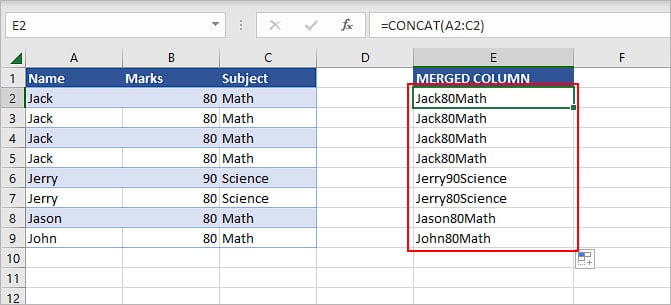
Now, use the Flash fill or drag handle to merge other columns.
Step 2: Create the Necessary Columns
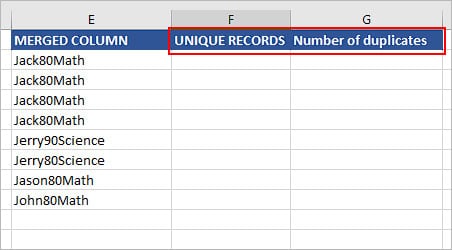
Create two helper columns to extract the unique records and list the number of duplicate records for each record. Here, we have “Unique records” and “Number of duplicates”.
Step 3: Extract Unique Values
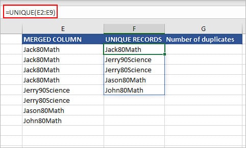
To get the unique records, you can use the UNIQUE function.
First, type =UNIQUE( and select the cell range of the merged column. Then, enclose it with the round bracket and press Enter.
Step 4: Count Duplicates
Now, to count the number of duplicate records, use the COUNTIF function similar to how we calculated for a single column in CASE 2.
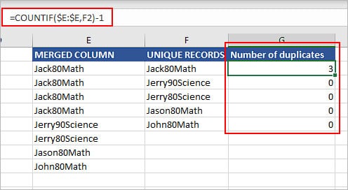
In the above image, we checked for the occurrence of Jack80Math in the entire “Merged Column” column. Notice that we used Jack80Math inside the Unique Records column as we only want to count the frequency of duplicate records once only.