Cell referencing is one of the key concepts you should master, preferably in the early stages of learning Excel. It determines which cell to refer to when copying and applying a formula.
Generally, Excel uses three basic types of cell referencing, which are relative, absolute, and mixed. Except for the relative referencing, the other two use dollar signs in the formula to lock the row, column, or both.
In a nutshell, cell referencing is all about whether you use the dollar sign and where you place it on the cell reference.
Relative Reference
Since all cell references are relative by default, chances are you use them most of the time in your formulas—whether knowingly or unknowingly.
The way it works is by adjusting the position of the row/column of the cell reference in the formula. So, both the column and row may change while pasting the formula to another cell.
For instance,
Here, the first sum is calculated in cell C2 using the formula =A2+B2. Now, when we copy its formula to other cells (C3 to C6), Excel uses relative referencing and shifts by row one while calculating the sum.
To visualize which cells are being used in each formula for cells in column C, you can turn on the Trace Precedents feature under the Formulas tab.
Absolute Reference
The absolute reference fixes both the column and row while pasting a formula on any cell on the worksheet. These are particularly useful when you want to use a formula across row/column while still using the same value stored on a particular cell.
You can convert a relative reference to an absolute one by adding a dollar sign before both the row and column such as $A$2.
For instance,
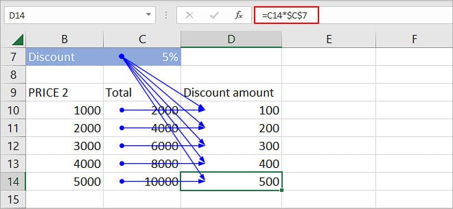
Here, we want to apply the discount to the total and calculate the discount amount. So, we used the formula, Total * Discount in the D10 cell.
However, we can notice that the rows are also shifting whenever other cells in “Discount Amount” (specifically cells D11, D12, D13, and D14) are using the formula from cell D10.
Therefore, we need to lock the C7 cell with the 5% value at the same position. We can do so by adding a dollar sign before its row and column after which the formula becomes =C14*$C$7.
And as shown in the image below, each cell in the Discount amount column is using the same cell reference; C7 in their formulas.

Likewise, if we copy the formula to the next column (Column E), notice that it’s still using the same C7 cell.
In a nutshell, absolute referencing prevents any cell (C7 in this case) from shifting both row-wise and column-wise while copying the formulas in other cells.
Mixed Reference
Mixed references are used in specific scenarios such as fixing only a row/column part of the cell reference.
It’s a bit complicated as you have to know which part of the cell reference should be locked to get the correct formula.
It is of the following two types.
Fixed Column, Relative Row
Here, we want to fix the column, but still be able to change the cell reference when we copy the formula across the rows.
For example: $A2
Fixed Row, Relative Column
Here, we want to lock the row and prevent Excel from changing it while copying the formula down the column. However, we still want to shift the column.
For example: A$2
Let’s take a look at an example that involves using both mixed cell reference types.
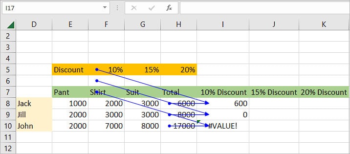
Here, we are trying to calculate the discount price after applying three discount rates; 10,15, and 20.
Initially, we want to calculate how much discount will each of our customers get after applying a 10% discount on their total price.

As expected, the relative reference didn’t work while copying the formula =H8*F5 for other cells. That’s because the cell with the 10% discount (F5) is shifting to the next row by one while calculating for each cell in the “10% Discount” column.
To fix this issue, we need to lock the F5 cell such that it doesn’t shift downwards in the formula. So, we lock the row part only. Therefore the formula becomes =H8*F$5 and the result is as follows.
Now, we want to calculate the discount price after applying 15% and 20% discounts. But, if we apply the current formula =H8*F$5, we can see that the Totals column isn’t fixed in the image below.
To solve this issue, we need to lock the Total column, which happens to be the H column for us. So, the formula becomes =$H8*F$5 and the result is as follows.
Summary
The whole cell referencing can be summarized as follows.
| Cell reference | Type |
| A1 | Relative cell reference |
| $A$1 | Absolute cell reference |
| $A1 | Fixed column, relative row |
| A$1 | Relative column, fixed row |
Other Cell References
While the above cell references are the major ones, there are two other cell references you might come across when working in Excel.
Circular Reference
You will see this specifically in an Excel error message. The circular reference is a cell reference that includes itself in the formula.
Structural References
When you reference any cell of a table in a formula, whether inside or outside of the table, Excel uses a special cell reference called the structural reference.
Here, instead of using general cell references with column and row names, like A2, Excel uses table and column names. As we are using names, a cell reference becomes more understandable and easy to remember.
For instance,
=SUM(tbl_Employee[Salary])
Even without knowing which cells are involved in the formula, it’s quite intuitive that the above formula has something to do with adding salary in the Employee table.