Previously, we learned how to create a Calendar in Excel from scratch. But, it would be tedious to add a Calendar manually every time you need to update an event, isn’t it? So, can you generate an automatic calendar and make it more interactive?
Well, the answer is absolutely Yes! I would definitely say Automatic Calendars are the Game changer when it comes to enhancing both your work efficiency and productivity skills.
In addition to constructing a dynamic calendar, we will also guide you on how to link it with your Task/Project Schedules and auto-update them together. So, Keep Reading!
As an example, I will create a monthly calendar for the Year 2024. I’ll include a few national and international events per the US Calendar.
Preliminary Step
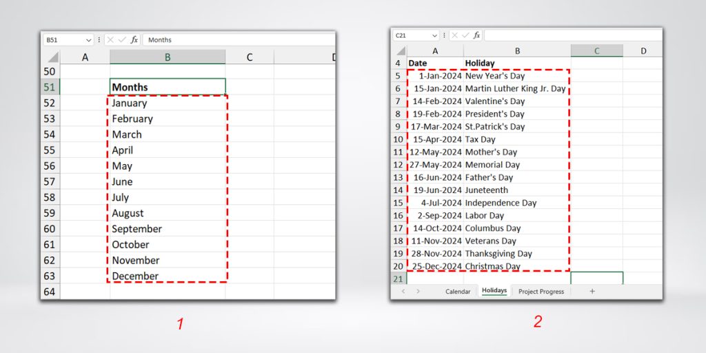
- Months Name: Create a list of months to prepare a drop-down list. Here, I have Months name in cell B52:B63 which is on the same sheet. It’s up to you if you want to input and reference the Month’s name in a Different Sheet.
- Holidays/Events: Make a list of Events to mark them as Holidays. Again, either enter in the same sheet or a different Sheet. This time I’ve compiled lists on a separate sheet.
Step 1: Prepare a Calendar Layout
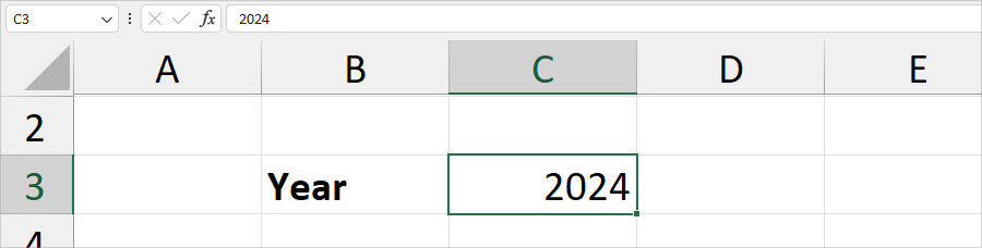
For the Calendar Layout and to input the Array Formula, we need the Year, Month names, Month Number, and First Day of the Month.
- Enter a Year in the cell.
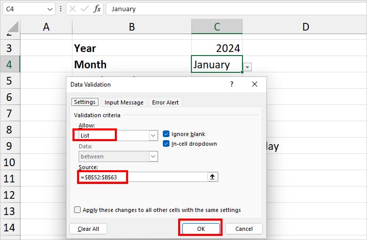
- Just below that cell, input Month and create a Drop-down list next to it. On the Data tab, click on Data Validation in the Data Tools group. Be on the Settings Tab and for Allow, pick List. Then, on Source, select the Month Name List.
- Under the Month cell, type in Month Number as a heading. Then, enter this formula
=MATCH(C4, B52:B63, 0)in the same row to return the month number. Here, the MATCH function returns the month number from B52:B63(Month Lists) for the lookup value of C4 (Month Name). For January, we got 1.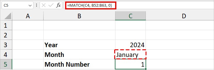
- Now, let us find the first day of the Month. For this, enter
=WEEKDAY(DATE(C3, C5, 1))the formula. It’ll return the Weekday number where the first day starts from. Since we got 2, it means the 1st Date is on Monday.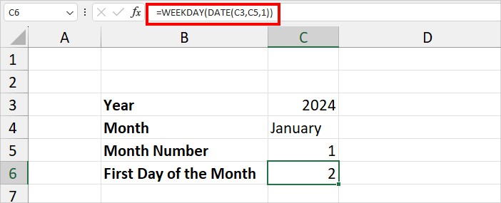
Step 2: Use the Formula to Enter Date
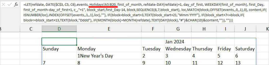
Now, once we have all the required information, enter the formula mentioned in the box. I know the formula can look advanced and intimidating. But, this is an array formula that’ll return all dates at once.
=LET(refdate, DATE($C$3, C5, C6),events, Holidays!A5:B20, first_of_month, refdate-DAY(refdate)+1, day_of_first, WEEKDAY(first_of_month), first_Day,first_of_month-day_of_first+1, c_,"+1", block_start,first_Day-14, block,SEQUENCE(8,7,block_start), loc,MATCH(block,OFFSET(events,,0,,1),0), content,IF(ISNUMBER(loc),INDEX(OFFSET(events,,1,,1),loc),""), IF(block=block_start+3,TEXT(block_start+21,"Mmm YYYY"), IF(block_start+7<=block,IF(block<=block_start+13,TEXT(block,"Dddd"), IF(MONTH(block)=MONTH(refdate),TEXT(DAY(block),"#")&CHAR(10)&content,"")),"")))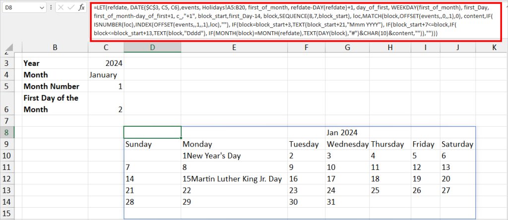
After you paste the formula, you might need to change a few cell references as per your data.
- On the DATE() function, cell C3 is the Year, C5 is the Month Number, and C6 is the First Day of the Month. Input the cell reference accordingly.
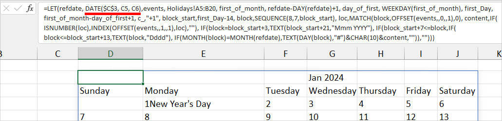
- Similarly, the fourth argument of the LET function, (Holidays!A5:B20) is events that are included in the Calendar. So, select your Holiday/Event Cell ranges.
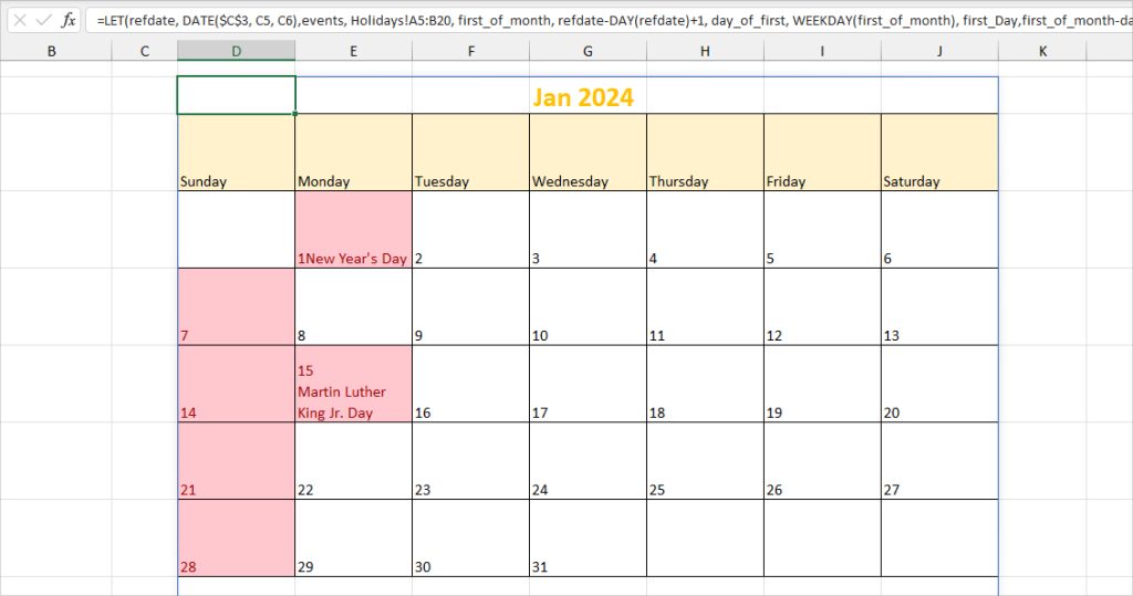
Step 3: Apply Formatting to the Calendar
Once you’re done, now, you can check out these tips to format the calendar.
- Expand the Row Height and Column Width.
- Select the Calendar area and use All Borders from the Font Tab to darken the gridlines.
- Change the Font Type, Colour, and Size as you wish.
- Highlight all the Cells with Dates that have Holidays.
Congratulations! You’ve just created an Automatic Calendar.
If you want to see another month, expand the drop-down menu for Month. Then, pick a different month. The Calendar will auto-update according to the chosen Month.
Similarly, the Calendar will also update automatically when you switch the Year.
Step 4: Link Calendar to your Project Schedule
After you have a dynamic Calendar, you can now link it to your Project Schedule. Keep in mind that this step is completely optional. But, creating a dynamic project schedule would make your work a lot more organized and keep it professional.
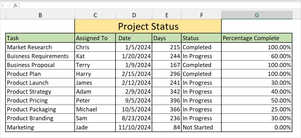
Let’s assume this is my Project Status. Using the FILTER function, we will return this in our Calendar Sheet.
- Firstly, on a new cell of the same sheet, enter the Start Date heading. Then, type this
=DATEVALUE("1-"&C4&"-"&C3)formula to return the date. Here, C4 is the month name and C3 is the Year. We are directly linking cells to make it dynamic.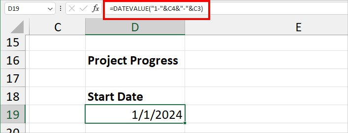
- Next, enter the End Date title. For the date, use the
=EOMONTH(D19, 0)formula. Here, D19 is the Start Date cell and 0 months is the end of the month.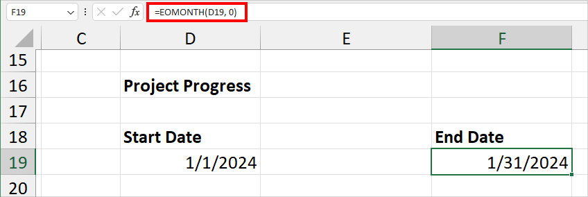
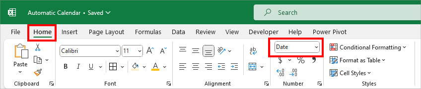
- If both the DATEVALUE and EOMONTH return the date in serial numbers, change the formatting to the Short Date from the Home Tab.
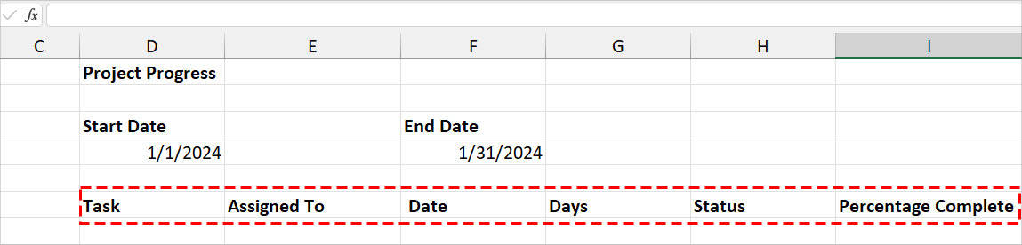
- Now, Copy-Paste the Project Schedule Titles from the original sheet like Task, Assigned To, Status, and so on.
- Below the title, enter this formula,
=FILTER('Project Progress'!B:G, ('Project Progress'!D:D>=Calendar!D19)*('Project Progress'!D:D<=Calendar!F19), "No Task"). The formula returns an array of Task Schedules from Project Progress which is >=Start Date and <=End Date.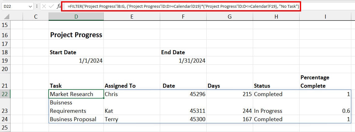
Once you’ve performed all these steps, you’ll now have a dynamic calendar as well as a project schedule.
When you change the month in the drop-down list of cell C4, the project status will show the task details for only that month. In case there are no tasks for the month, it’ll show “No Task.”