By default, Excel uses relative cell referencing to copy formulas across rows or columns. So, you are knowingly or unknowingly using it most of the time when copying and pasting formulas to other cells.
However, it may not be appropriate all the time. In some cases, you would want to fix a cell in the formula no matter where you are copying it. That’s where you need to convert the regular relative cell reference to an absolute cell reference.
What is Absolute Reference?
A cell reference whose rows or columns are locked in one place and won’t change when copying a formula to other cells is known as an absolute cell reference. This prevents a reference to move as the formula is copied.
Let’s take a look at an example to better understand the concept.
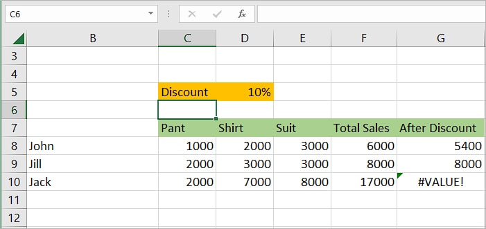
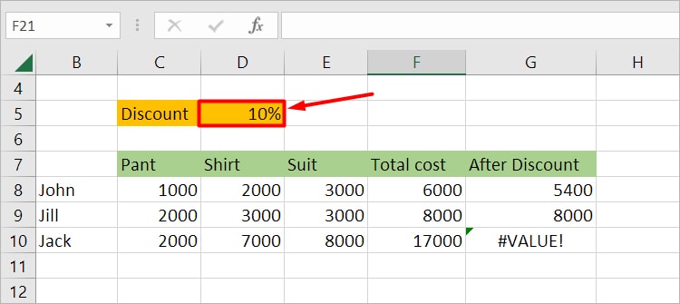
Here, we have three customers (John, Jill, Jack) who bought some clothes (pants, shirt, suit) from our store.
And, we want to calculate the actual price after applying the discount on the total cost. For this, we are using the following formula:
Total cost -Discount * Total cost
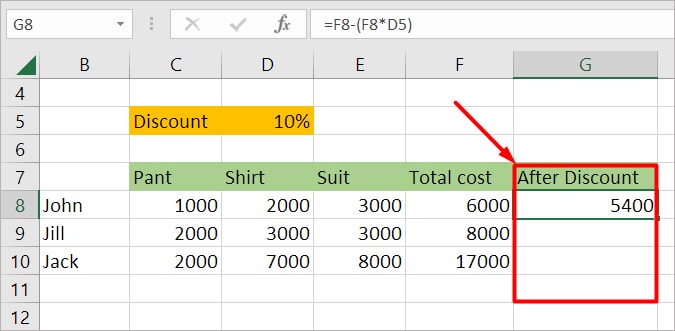
Now, please take a look at the above image, specifically under the After Discount column.
Then, try to guess what would be the result if we copied the formula on the G8 cell for other cells, G9 and G10, below it.
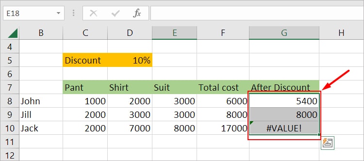
Well, as you can see, other cells are not using the correct formula. One cell even resulted in a #VALUE! Error.
So, what’s going on? How is Excel calculating other cell values?
As we mentioned earlier, Excel uses relative cell referencing by default. So, as we copied the formula down the column, the cell with the Discount value (D5) also started to shift downwards because of it.
To visualize which cells are being used in each formula for the G9 and G10 cells, you can use the feature called the Trace Precedents option. You can find it under the Formula tab inside the Formula Auditing section.
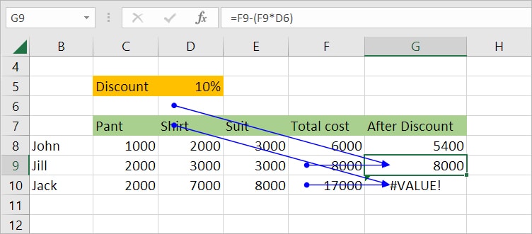
Now, you can notice that the D5 cell isn’t fixed for other cells G9 and G10 as we expected.
The formula for G9 is currently =F9-(F9*D6). But, since the D6 cell is empty, the formula =F9-(F9*D6) leads to =8000*8000-0 and the final result is 8000. Also, the G10 cell returned an error because it tried using the text “Shirt” with a number in its formula.
So, how do we fix it?
In a nutshell, we want to lock the D5 cell which contains our discount value such that whenever we copy the formula, it moves neither across the row nor down the column. In such cases, we need absolute cell referencing.
How to Use Absolute Reference?
To use absolute cell referencing in your formula, follow the steps below.
- Select the cell which contains the formula and needs absolute cell referencing. In our case, it’s one with the discount value.
- Double-click to enter the Edit mode. Or, use the formula bar. One important tip is that always fix the first cell where you copy the formula from.
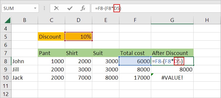
- Place the cursor on the cell reference you want to change.
- Insert the dollar sign before both the column and row. Or, simply press the F4 key to cycle through different cell reference types and stop when you see the two dollar signs.
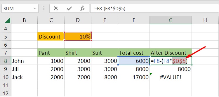
- Press Enter.
- To convert other cells into an absolute cell reference, just repeat Step 4.
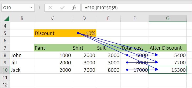
After we used absolute referencing, all other cells only use D5 in their formulas as shown in the image below.
Note: Some laptops assign the F4 key to use the media controls. In such cases, you have to press Fn + F4 to cycle through the cell reference types.Ways to Absolute Reference
While you can use absolute referencing to lock both the column and row part of a cell reference such as $A$2, you can choose to lock it partially.
For that, you just need to add the dollar sign before it.
For instance,
- If you just want to lock the column and not the row, you would have a cell reference such as
$A2. - Similarly, to lock only the row, place the dollar sign in front of the row part, such as
A$2.