VSTACK is a comparatively new function available in Excel 365 and Excel web. VSTACK dynamically piles arrays passed as arguments in the formula. VSTACK supports 3D-referencing and is the best function to use when trying to summarize multiple sheets into a single worksheet.
In this article, we will be discussing the arguments used in the VSTACK function and put it into application to see how it works nested with or without other functions in a formula.
Arguments Used in the VSTACK Function
VSTACK is used in the following format while constructing a formula:
=VSTACK(array1, [array2],...)- array1: The first array you wish to stack on top of the array.
- array2: The other arrays you wish to stack below the first arrow.
You can add up to 60 arguments inside the VSTACK function. It is mandatory for you to enter the first array while the remaining arrays are optional.
VSTACK in Application
VSTACK is a great alternative to copy-pasting data from other tables or worksheets. This is because VSTACK is dynamic and for any data you add or remove in the range, the function automatically updates the information.
Example 1: Merge Tables Inside a Worksheet Using VSTACK
In this spreadsheet, we have two data tables. Let’s merge these tables into one singular table that holds information from both of these arrays.
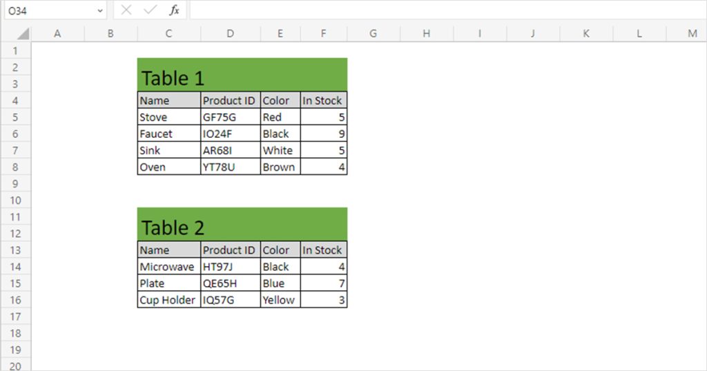
In cell H3, I entered the VSTACK function in the following formula:
=VSTACK(C4:F8,C14)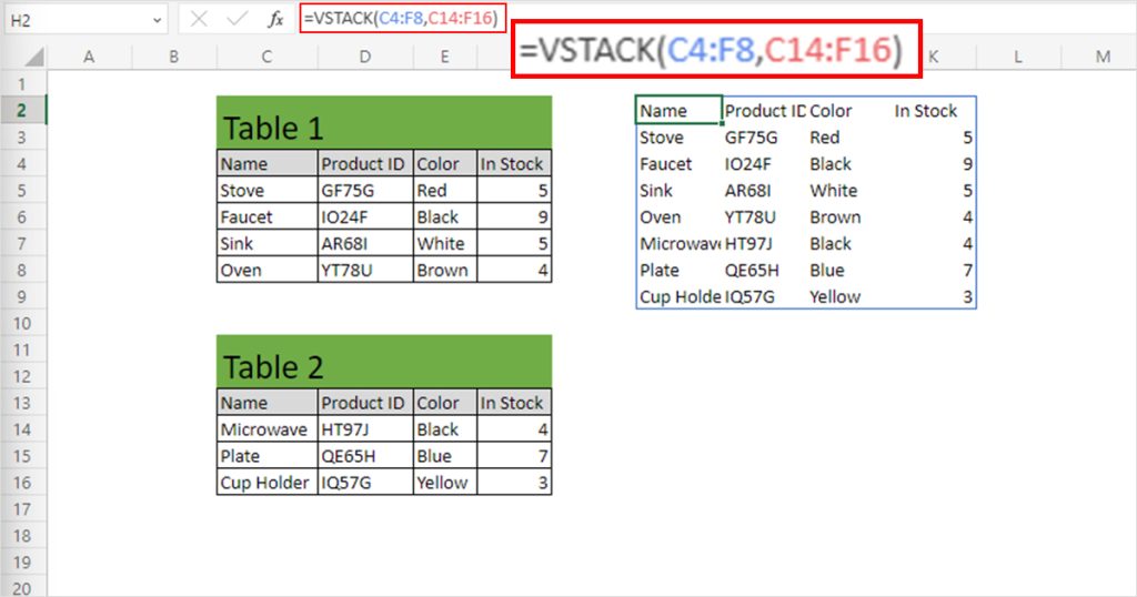
I will now use the format painter to copy the formatting I had applied in the tables I just merged.
Example 2: Merge Data in Multiple Worksheets Using VSTACK
Say you have a workbook with the sales data for the entire year. You can merge all of these data into one worksheet using the VSTACK function.
In the following spreadsheet, we will be using the VSTACK function to create a 3D reference to integrate data in these worksheets into one dynamically.
We first started by creating a new worksheet. In cell A1, we entered the following formula:
=VSTACK(January!A2:AF11,February!A2:AF11,March!A2:AF11,April!A2:AF11,May!A2:AF11,June!A2:AF11,July!A2:AF11,August!A2:AF11,September!A2:AF11,October!A2:AF11,November!A2:AF11,December!A2:AF11)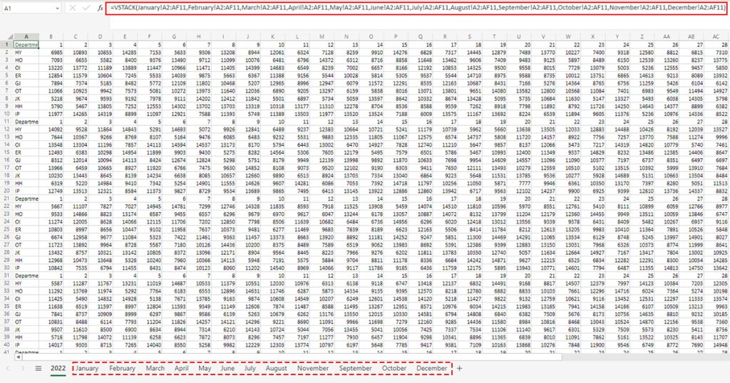
I know, the formula looks HUGE! But don’t worry, we’ve just referenced 12 worksheets and the range we wish VSTACK to retrieve the data from. If you have a bigger data sheet to reference like this, hold on to the SHIFT key and select the worksheets you want to reference.
If you want to reference an entire workbook, hold down the SHIFT key and select the last workbook. However, do not do this if you’ve created a worksheet in the current workbook as it will create a circular reference, causing your formula to not work.
Example 3: Include Headers on the Stacked Data
You can include text headers on top of your stacked data. All you have to do is enter the data as a text array and then pass your ranges.
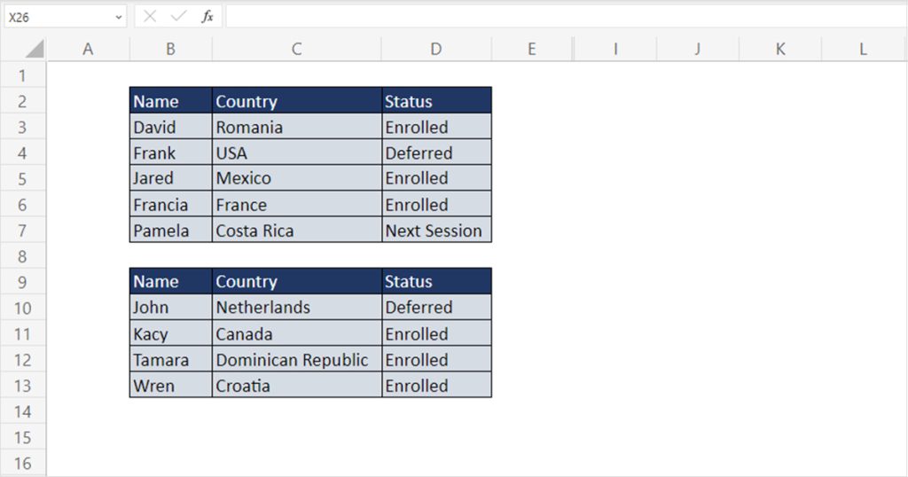
Let’s concatenate Array 1 and Array 2 into a single array. On top of these data, we will be giving three headers named, “Name”, “Address”, and “Status”.
In cell F2, we entered the following formula:
=VSTACK({"Name","Country","Status"},B3:D7,B10:D13)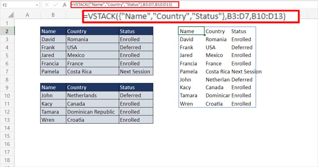
VSTACK will spill the data from the range B3:D7 and B10:D13 under our text headers.
Example 4: Nesting Functions with VSTACK
You can nest other functions using the VSTACK function. In my experience, I always nest VSTACK under the IFERROR function.
When VSTACK cannot find information in the given range, it results in an #N/A error. There may be slots you’ve left empty to fill in the future, or there may be no data to put in the first place.
Errors never look good on a worksheet. Therefore, the IFERROR function comes in handy to give Excel an idea of what to enter if the formula results in any error. This is how you can incorporate the IFERROR function with VSTACK:
=IFERROR(VSTACK(range),(value if there’s an error))Whatever you enter in the value if there’s an error section is the data Excel will return when you get an error.