VLOOKUP is a powerful lookup function in Excel. You can use VLOOKUP to look up values vertically in the same row, but different columns. Unfortunately, VLOOKUP comes with its own limitations. For starters, you cannot set multiple conditions for when you want to look a value up from the range.
If you wish to use VLOOKUP, you need to create a unique lookup value. In this article, we’ve gathered steps you can use to create a unique lookup value when you have multiple criteria.
If you’re an Excel 365 user, you can also look into using XLOOKUP as an alternative method of looking up values with multiple criteria. You can use the boolean logic to set multiple criteria in XLOOKUP, therefore this method is swifter.
How to Use VLOOKUP
Before we jump ahead to learn how you can use VLOOKUP with multiple criteria, let’s understand the basic functioning of the VLOOKUP function.
Here are the arguments VLOOKUP uses when constructing a formula:
=VLOOKUP(lookup_value, table_array, col_index_no, [lookup_range])Here is a quick breakdown of what these arguments mean:
- lookup_value: VLOOKUP will return the data corresponding to this value.
- table_array: The range to look value from. Both, your lookup_value and the return value should fall under this range.
- col_index_no: Enter the column number of your return value. The value must be relative to the table_array and not the entire grid.
- [lookup_range]: Enter TRUE for VLOOKUP to return the closest value and FALSE for it to return the exact value.
For better understanding, here is an example using VLOOKUP the traditional way. In this sheet, we’re looking at the total sales made by an employee at a company for the month of January. Let’s use VLOOKUP to look up what percentage of commission an employee took for the month.
=VLOOKUP(H3,A1:E11,5,FALSE)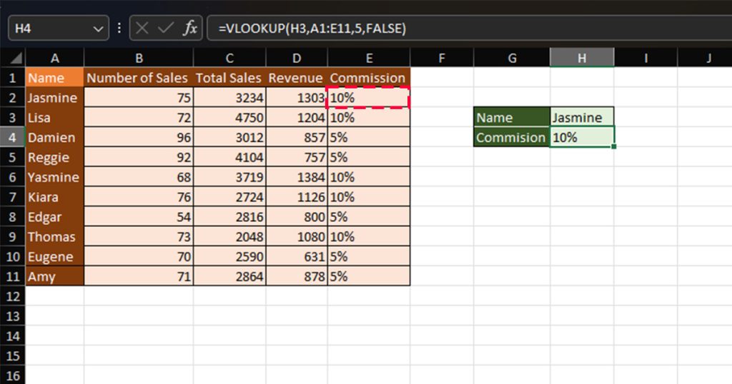
In this formula, our lookup_value is H3 which holds the value, Jasmine. VLOOKUP will give us the value corresponding to Jasmine. Our table_array is A1:E11. This is the area VLOOKUP will look for value in. The col_index_number is 5 so, VLOOKUP will extract value from the fifth column of the table_array, corresponding to Jasmine in row two.
Lastly, [lookup_range] is FALSE, meaning we’re looking for an exact match.
Here is what happened when we ran the formula.
Use VLOOKUP with Multiple Criteria
By default, you can only use one criteria in VLOOKUP. However, we can work around this issue by creating a helper column.

In this example, we’re looking for the Review on Product: T-shirt, and earmuffs for a list of 12 customers. As you may notice, the same name has been repeated twice. If we use VLOOKUP conventionally, it will only consider the value from the Review column for the first name. As a workaround, we’ve changed the lookup_value to the value we concatenated.
Step 1: Create a New Column
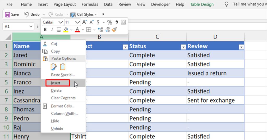
You will have to create a column to concatenate the names with the products. Right-click on column A and select Insert. Make sure that the new, concatenated column is the first column in the spreadsheet, or else you’ll run into the #N/A error.
Step 2: Concatenate Name and Product
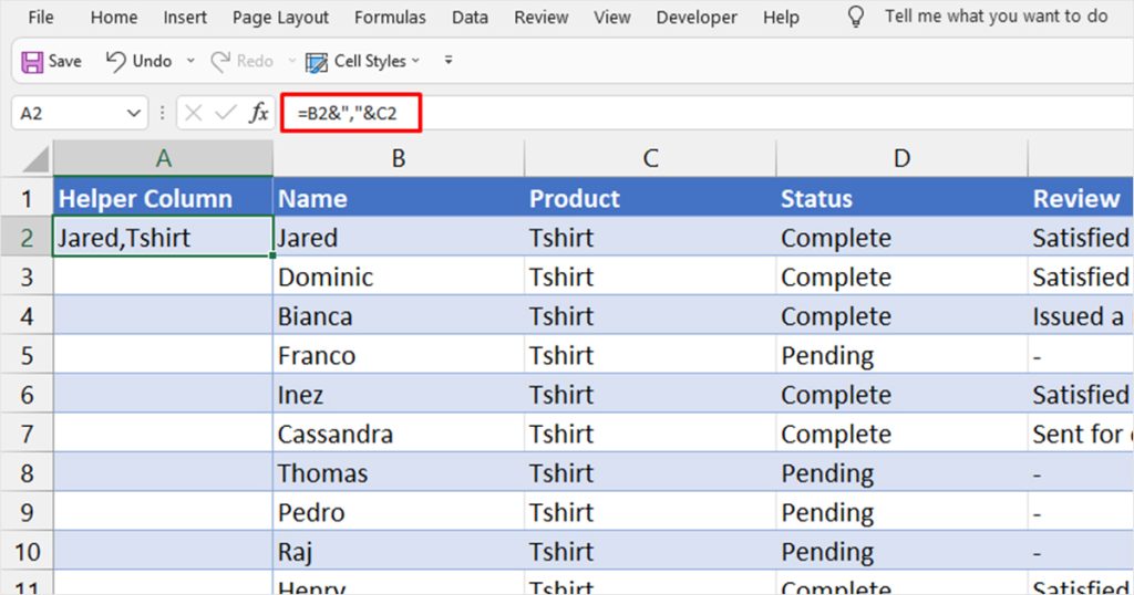
To concatenate, we simply used the Ampersand operator. On column A1, we’ve entered =B1&","&C1 to merge column Name and Product. We used commas as a separator between these two cells.
Step 3: Use the VLOOKUP Function
Now that we have unique lookup values, we can use the VLOOKUP function, normally. Using the general format, we’ve entered the formulas as
=VLOOKUP(H8&","&C2, A2:E25, 5, FALSE)
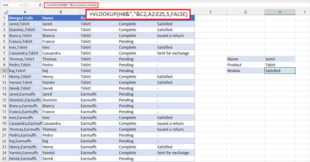
The VLOOKUP formula will look for the exact value corresponding to the value, “Jared,Tshirt” in column three, which is the Review column.
This formula returns, “Satisfied” which is the review given by Jared on the item, Tshirt.
Alternatives to Using VLOOKUP
It can be a rather tedious task to create a helper column each time you wish to look up a value with multiple criteria. Therefore, you can use a quicker alternative which is to use XLOOKUP instead of VLOOKUP.
Use XLOOKUP with Multiple Criteria
If you’re using Excel 365 or the web version of MS Excel, you will have the option to use XLOOKUP. XLOOKUP is similar to VLOOKUP, however, instead of looking for values just vertically, XLOOKUP looks through values both horizontally and vertically.
You can use boolean logic to construct the XLOOKUP formula that considers multiple criteria. A BOOLEAN value either returns TRUE or FALSE. Numerically, these values translate to 1 and 0 respectively.
Writing it into a formula would look something like this:
=XLOOKUP(1,(condition1)*(condition2),(return array))Here is an example to better explain this formula. In this spreadsheet, we’re looking at the sales sheet for a company. Multiple employees can have the same name, however, they have a unique employee ID. We will be using the employee’s name and employee ID to look up the percentage of commission they received for the month.
We’re looking to view the commission of the employee named Jasmine with Employee ID 000-040. To generate the result, we have written the following formula:
=XLOOKUP(1,(B2:B51=I5)*(A2:A51=H5),E2:E51)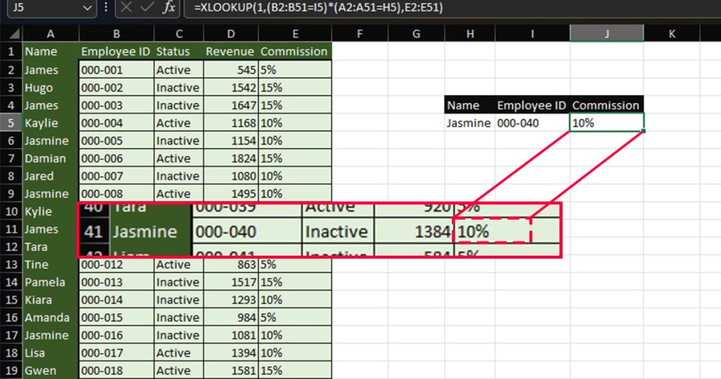
| Formula | Description |
B2:B41=I5 | In the range B2:B51, looks for the value that is equal to cell I5, 000-040. Once this criterion is met, it becomes a TRUE condition and returns 1. |
A2:A51=H5 | In the range A2:A51, looks for the value that is equal to cell H5, Jasmine. Once this criterion is met, it becomes a TRUE condition and returns 1. |
(B2:B51=I5)*(A2:A51=H5) | When B2:B41 and A2:A51 are TRUE, this formula returns 1. |
XLOOKUP(1,(B2:B51=I5)*(A2:A51=H5),E2:E41) | Once the condition returns 1, XLOOKUP with return the corresponding value from the range E2:E51. |