Lookup functions like VLOOKUPs have made it so much easier to pull out values from a different sheet.
However, since the VLOOKUP itself is an advanced function, adding extra sheet referencing to the formula can be a little confusing – for most beginners.
Here’s a simple formula that might quickly help you understand the VLOOKUP Between Two Sheets.
=VLOOKUP(lookup_value, SheetName!table_array, col_index_num, [range_lookup])In the above formula, every function argument is pretty much the same as how you would normally use VLOOKUP. The only difference is we are taking a table array reference from another sheet.
To use this function across two sheets at its utmost potential, I have also discussed how to make it more dynamic at the end of this article. So, Keep Reading!
VLOOKUP Between Two Sheets in the Same Workbook
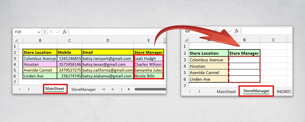
Suppose, I need to draw out the value from MainSheet to the StoreManager Sheet of the Same Workbook as shown in the image.
For that, I’ll enter the formula as
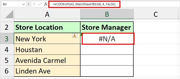
=VLOOKUP(A3, MainSheet!B3:E6, 4, FALSE) 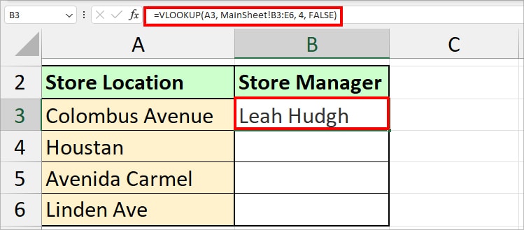
In the formula, A3 (Colombus Avenue) is our lookup value. The VLOOKUP will return the item from the 4th column of the B3:E6 cell range in MainSheet.
Since we specified a FALSE argument, it returns the exact match. I got Leah Hudgh.
Once you get the result, you can always use the Flash-Fill Handle for the rest of the columns. It’s the fastest way to extract data from another source, isn’t it?
While you can manually type this formula, I wouldn’t quite recommend doing so. This is because, again, you would have to remember the cell ranges, columns, and so on to input the arguments.
Instead, use this method and easily use the VLOOKUP function.
- In the result cell, type =VLOOKUP and click on the Lookup cell. Then, enter a comma (,). For example, =VLOOKUP(A3,
- Now, head to Another worksheet and select the cell ranges. Then, Put a comma and enter the Column Index Number. Again, put a comma and type the TRUE or FALSE argument.
- Finally, close the Bracket and press Enter. You will have the value in the result cell.
I believe you must have gotten an idea of how to do VLOOKUP between two different worksheets. But, let’s take a look at more examples.
| Example | Formula | Description |
| Table Data | =VLOOKUP(C10, Table1, 2, 0) | Our Lookup Table is in Table Format. Its name is Table1. For Table Range, the VLOOKUP will not display the Sheet name. |
| Named Range | =VLOOKUP(A3, ShopInformation, 4, 0) | Here, ShopInformation is our Named Range for the Lookup Table. Again, here, no Sheet Name. |
Nested VLOOKUP Functions Between Two Sheets
You can nest the VLOOKUP and other functions like IFERROR and INDIRECT to manipulate the formula. It can be handy when you want to address cell errors or make sheet referencing less complicated.
VLOOKUP and IFERROR Function
Is your VLOOKUP resulting in cell error?
This can happen due to a number of reasons. However, if it results in a #N/A error because there is no lookup value in the lookup table, there’s a workaround.
With IFERROR and VLOOKUP together, you can dodge such cell errors and replace them with “Any value of your choice.”
Suppose, I got a #N/A error. Let’s return “No One” instead of the error in the spreadsheet.
For that, my formula would be
=IFERROR(VLOOKUP(A3, MainSheet!B3:E6, 4, FALSE), "No One")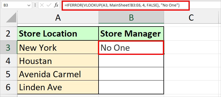
IFERROR, VLOOKUP, and INDIRECT Function
So far, we’ve been referencing the Sheets by manually selecting the cell ranges. But, this can go wrong when there is a large dataset.
Let’s make Sheet Referencing easier in the VLOOKUP formula. For that, we will nest the VLOOKUP with the INDIRECT Function. Also, to replace the error, we will again use the IFERROR.
Firstly, create a Named Range for your Lookup table. Assuming our Named Range is “Store_Location,” I used this formula.
=IFERROR(VLOOKUP(D2, INDIRECT("Store_Location"), 2, FALSE), "Not Found")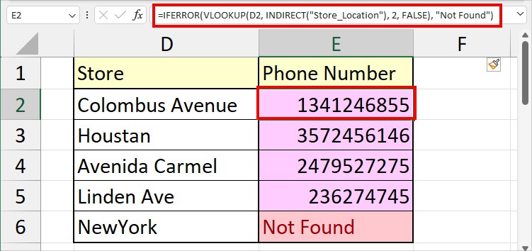
In this formula, INDIRECT(“Store_Location”) is our table array in the Main Sheet.
VLOOKUP Between Two Sheets in Different Workbooks
Now, we will look into the VLOOKUP between two sheets in two different workbooks.
For that, our VLOOKUP formula would be
=VLOOKUP(lookup_value, [Workbook.xlx]SheetName!table_array, col_index_num, [range_lookup])Remember to open the source and destination workbook before using the formula.
Example:
Here, I will extract the Email Column from Sheet 5 of the Suppliers Workbook to Sheet 4 of the Batsy workbook.
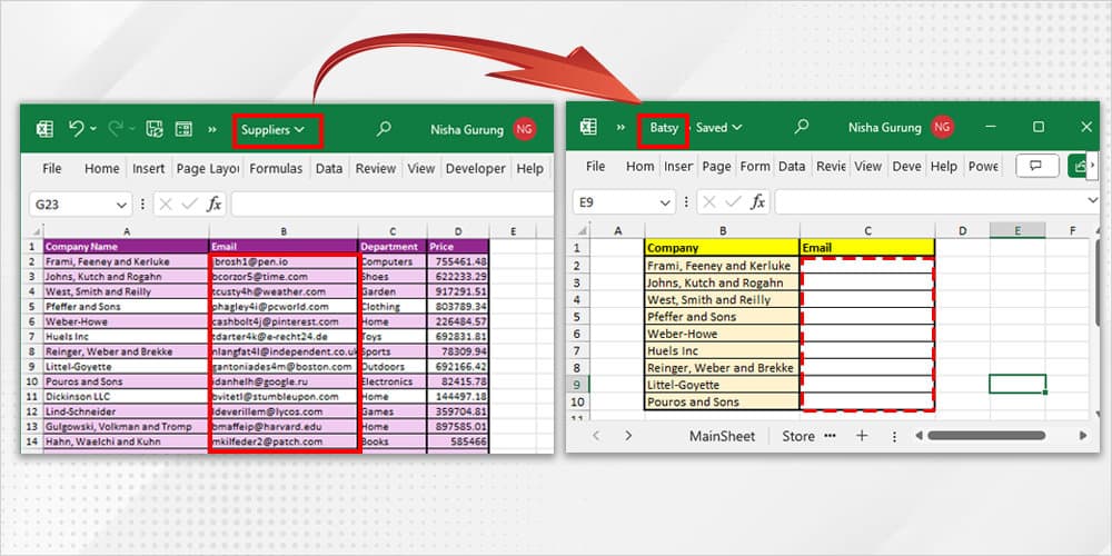
I used this formula to return the data.
=VLOOKUP(B2, [Suppliers.xlsm]Sheet5!$A$2:$D$21, 2, 0)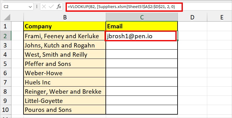
To enter the formula, I first set my two Excel workbooks in Side by Side View. Then, in the destination workbook, I typed the =VLOOKUP(B2 argument. After that, I headed to another workbook, selected the cell ranges, and entered the remaining arguments.
Can You Make VLOOKUP Between Two Sheets More Dynamic?
Yes, you can also make the VLOOKUP Between Two Sheets more dynamic just like how we do within the same sheet.
Suppose I need to create a fillable form in Excel. This time, in my Main Sheet, I have the form. In the second sheet, I have Additional store information like Mobile, Email, Supervisor, etc.
If my participant picks any Location option in the Form, I want to return all information related to it from the Second sheet.
For this, I will insert a drop-down list and use the VLOOKUP formula between the two sheets.
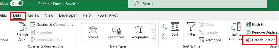
- Select a cell and click on Data Validation from the Data Tab.
- Pick List in the Allow option. Using the collapse icon, pick a Source and hit OK. Here, my source is in
=Sheet5!$B:$B. I have referenced the entire column such that the drop-down lists will take the newly added cells too.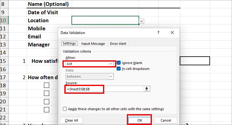
- Now, enter the VLOOKUP formula as
=VLOOKUP($C$10, Sheet5!B2:E5, 2, 0).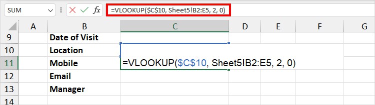
- Similarly, I used the same formula with a different Column Index for another column. Finally, if you pick a Value in the Drop-down list, the VLOOKUP will return values.