The UPPER function is a text function in Excel, used to convert all letters into upper case. The UPPER function works for texts and string values. While UPPER changes the case of alphabets in strings, numbers, and other symbols are left unchanged. This is also true for numeric and date values.
Arguments in UPPER Function
The UPPER function is a single parameter. This means you can only pass one value as an argument inside the function. You can pass a cell reference as the argument or even hard-code your argument.
When constructing a formula, use the UPPER function in the following format:
=UPPER(text)Applications of the UPPER Function
You can use the UPPER function to convert values such as codes, which are mostly in upper case. Similarly, as most documents require full names to be capitalized, you can use UPPER to change these text values without having to manually change their cases.
Example 1: Using a Reference as an Argument
You can use a reference as an argument for the UPPER function.
When you’re using a reference, you don’t have to worry about adding extra syntaxes inside the argument. However, remember that if you make any changes in the source cell, the change will be reflected in the referenced cell.

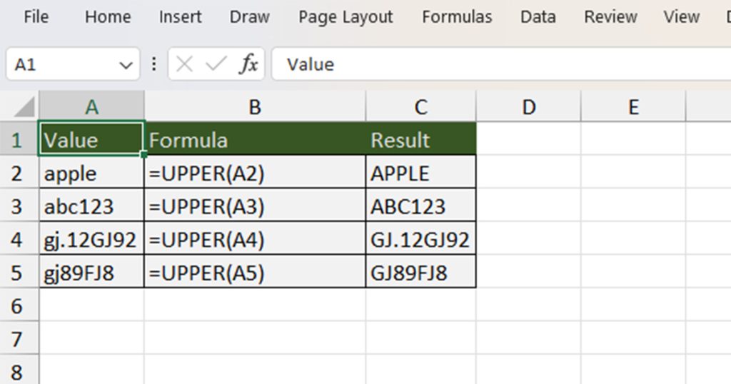
Here’s how you’ll construct a formula for each of these values using the UPPER function
| Cell Location | Value | Formula | Result |
| A2 | apple | =UPPER(A2) | APPLE |
| A3 | abc123 | =UPPER(A3) | ABC123 |
| A4 | gj.12GJ92 | =UPPER(A4) | GJ.12GJ92 |
| A5 | gj89FJ8 | =UPPER(A5) | GJ89FJ8 |
Example 2: Using Hard Code Values as Arguments
If you frequently make changes to your values in the spreadsheet, it is best if you hardcode your arguments in the UPPER function. While hard coding your value, you will have to enter your text or string in double quotes. If you skip this syntax, Excel will read the argument as a reference, and you will encounter the #NAME? error.

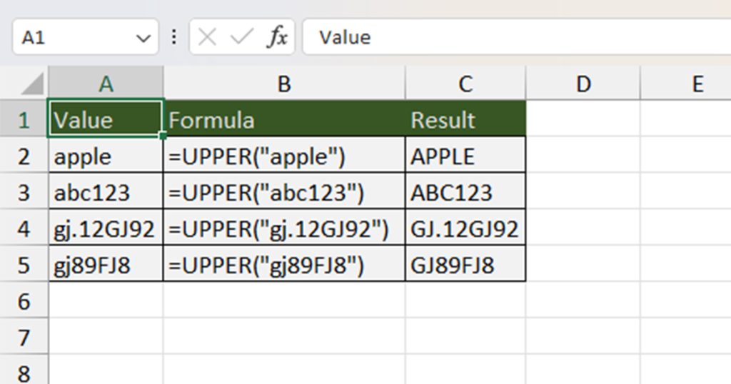
We used the same values we did in the first example. See how you can enter the formula to hardcode your values in the UPPER function:
| Value | Formula | Result |
| apple | =UPPER(“apple”) | APPLE |
| abc123 | =UPPER(“abc123”) | ABC123 |
| gj.12GJ92 | =UPPER(“gj.12GJ92”) | GJ.12GJ92 |
| gj89FJ8 | =UPPER(“gj89FJ8”) | GJ89FJ8 |
Other Applications of UPPER: Conditional Formatting
You can also use the UPPER functions to set rules in other features such as Conditional Formatting. Let’s assume you’re trying to highlight cells in a range that has a value in upper case. You can nest the UPPER function insider EXACT to the condition to format such cells.
Now, you can’t only use UPPER while setting this condition. This is because Excel, by default, is not case-sensitive. This means it will read apple and APPLE as the same thing. This is overcome by nesting UPPER inside EXACT, which is case-sensitive.
- Select the range with your values.
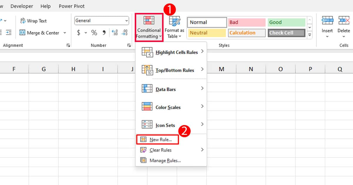
- Head to the Home tab.
- In the Styles section, select Conditional Formatting.
- Choose New Rules.

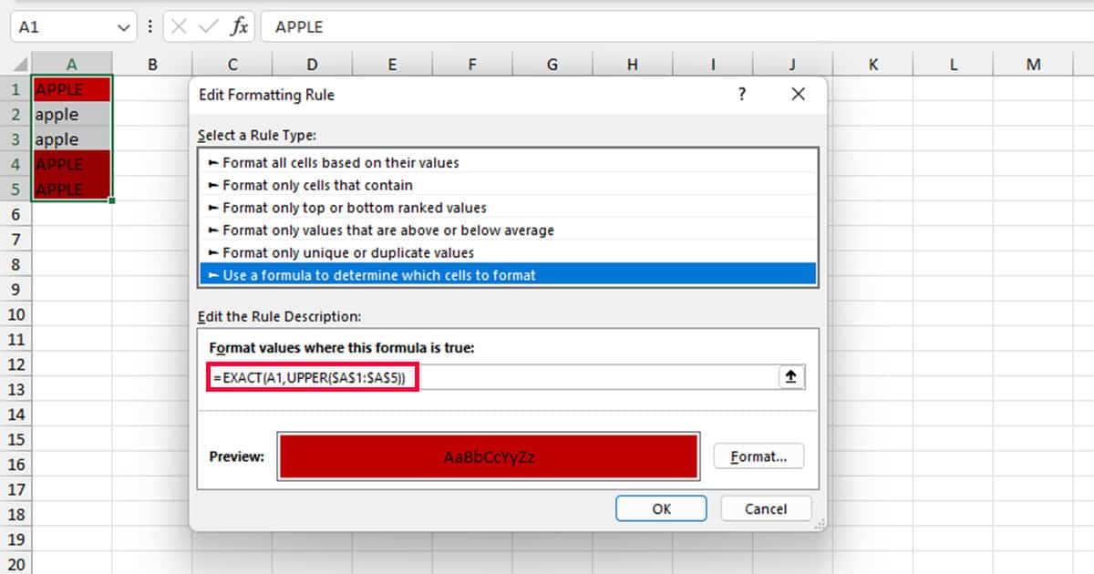
- Under Select a Rule Type, choose Use a formula to determine which cells to format.
- Under Format values where this formula is true, enter the formula in the following format:
=EXACT(UPPER(“(your value”), (cell range))- Click OK.

Similar Functions Like UPPER
There are two other functions like UPPER that change the cases of texts in Excel. All of these functions, like UPPER, are text functions and require only one argument as a parameter.
The LOWER function is the exact opposite of the UPPER function, which converts the case of all letters in a word into lowercase. Similarly, the next function is PROPER, which converts the initial of the set word into uppercase, leaving the remaining in lowercase.
Here are the syntaxes both functions use while constructing a formula in Excel: