If you have unnecessary spaces in your Excel data, you would have a hard time manually tracking and deleting them. But, Excel has an in-built function called “TRIM” to remove any extra spaces from the value.
Using the TRIM function, you could delete all irregular spaces while keeping the single ones. For Instance, the TRIM function returns the word ” Microsoft Excel ” as “Microsoft Excel.” You could also nest this function with other functions such as CONCAT, PROPER, LEN, etc. Let’s learn how to use the TRIM function from this article.
Arguments for a TRIM Function
TRIM function eliminates the extra spaces in text strings or words. You could use this to return only required single spaces on texts.
Syntax: TRIM(text)The TRIM function takes only texts as an argument. If you pass down a word or text string in the formula, you must place them inside the double quotation mark. For Instance, =TRIM(“text”). However, if you input a cell reference, you do not have to do so. Check out this example.

| Example | Formula | Result |
| Remove space in Excel | =TRIM(“Remove space in Excel”) | Remove space in Excel |
| Calculate Interest on Loan | =TRIM(A3) | Calculate Interest on Loan |
Applications of using TRIM Function
The TRIM function will remove all excess spaces from a text or words in Excel. But, if you wish to delete only the leading spaces, you can nest the TRIM function with other functions. Also, the TRIM function can be extremely useful when you are splitting or merging data in a spreadsheet. Let’s check out the applications of the TRIM function with the examples below.
Example 1: Remove Only Leading Spaces
In some instances, you may have an extra space in a text string on purpose. But, you might want to get rid of only the leading spaces from texts or numbers. Now, for this, we will nest the TRIM with other functions to delete only specified spaces.
Case 1: Text Strings
Suppose, you have Area Codes with leading spaces in Column A. The texts also contain double spaces between the code and the city. To remove just the leading space, you can enter the following formula.
=MID(A15, FIND(MID(TRIM(A15), 1, 1), A15), LEN(A15))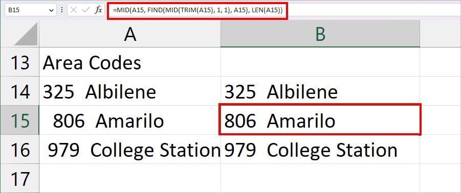
It’ll return 806 Amarilo as a result.
If you’re new to MID or LEN functions, the formula might appear complex to you. But, we will break down each of them and learn how it works.
- TRIM(A15): Firstly, TRIM(A15) returns the “806 Amarilo” value with stripped away spaces.
- MID(TRIM(A15), 1, 1): We have specified the MID function to return the 1 character from the 1st position. So, it will return the “8” string from “806 Amarilo”.
- FIND(MID(TRIM(A15), 1, 1), A15): This formula looks for the value of MID(TRIM(A15), 1, 1) which is “8” in cell A15 (“806 Amarilo”). Then, returns 3.
- MID(A15, FIND(MID(TRIM(A15), 1, 1), A15), LEN(A15)):
- Here, LEN(A15) formula counts the total number of characters of cell A15 value “ 806 Amarilo” including all spaces. Then, it returns 14.
- In MID function, we have passed down cell A15 as text, FIND(MID(TRIM(A15), 1, 1), A15) as Start_num, and LEN(A15) as Num_chars arguments. So, the MID function extracts all the characters starting from the 3rd position of cell A15. Thus, as a result, you get “806 Amarilo”.
Case 2: Numbers
The TRIM function returns the trimmed values in text format. So, if you only use the TRIM function to remove leading spaces from the numbers, it’ll format the values as text. When this happens, you’ll only receive 0 output for calculations. For Instance, while adding numbers using the SUM function.
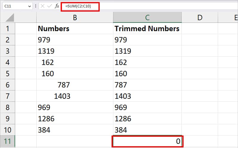
So, to trim numbers as well as return them in number format, we will nest the TRIM and VALUE functions together.
Let’s say, you have numbers with leading spaces in Column B. Now, to remove them and get the values in numbers, you need to enter the formula as
=VALUE(TRIM(B2))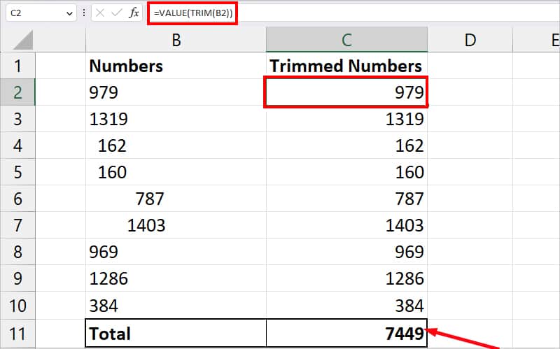
Firstly, the TRIM(B2) formula returns the number with eliminated spaces in the text. Then, the VALUE function converts the texts into number format.
Example 2: Extract Values
When you use certain functions like LEFT and RIGHT to extract the text strings for data, irregular spacing can return a different value than expected. This is because the formula also counts the space as a character.
For Instance, you have “ Table of Contents” text in the A6 cell. You want to extract the word Table using the LEFT function. For this, if you enter =LEFT(A6, 5), you’ll only get Tab. This is because there are two leading spaces in Table.
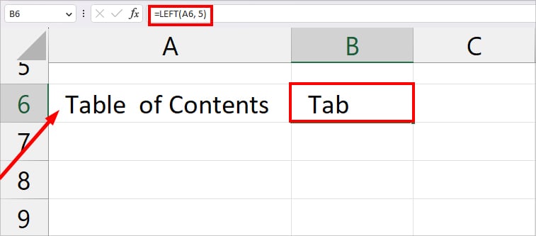
So, to eliminate leading spaces and extract the Table, you could nest the TRIM function inside the LEFT function. For this, enter the formula as
=LEFT(TRIM(A6), 5)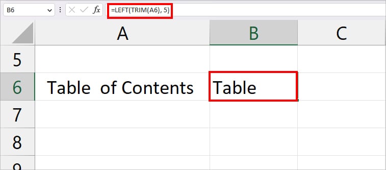
The formula first returns the text “Table of Contents” where all the unnecessary spaces are deleted. Then, the LEFT function returns 5 characters from “Table of Contents” which is Table.
Example 3: Use Trim While Merging Cells
Extra spaces can be equally troublesome while combining texts in Excel too. For example, you have “ 806” in the A2 cell and “ Amarilo” in B2 cell. If you used the =CONCAT(A2, " ", B2) formula, you’d get “ 806 Amarilo” in the result which contains a lot of unnecessary space.
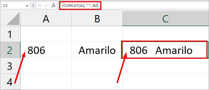
But, you can nest the CONCAT function inside the TRIM function to avoid this. You could use the formula mentioned in the box.
=TRIM(CONCAT(A2, " ", B2))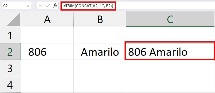
The above formula will first join the values of A2 and B2 and return “ 806 Amarilo”. Then, the TRIM function eliminates unwanted spaces from the result and returns “806 Amarilo” as a final output.
Example 4: Capitalize the First Letter of Word
Excel’s PROPER function can be used to return each first letter of the word in capital letters. In most cases, when you import the data, it may have lowercase and a lot of improper spacing. So, you could also nest the TRIM function inside the PROPER function. This way, you wouldn’t have to manually enter and adjust the spacing after capitalizing letters.
Let’s check out its uses with the given example. Suppose, you need to capitalize the value of cell A3. For this, your formula would be
=PROPER(TRIM(A3))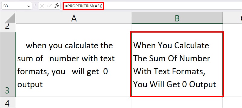
The TRIM(A3) formula first eliminates spaces from the value of A3. After this, the PROPER function capitalizes each first letter of the result.
Example 5: Count Total Number of Characters in Text String
In Excel, LEN functions are mostly used to count the total number of characters in a Text String. But, this function fails to exclude the unwanted spaces in the value. So, the TRIM function can also be useful to find out the accurate length of the text string with only a single space.
For Example, if you have “ Excel ” in cell A2 , =LEN(A2) will return 9. In this case, you can enter the given formula.
=LEN(TRIM(A2))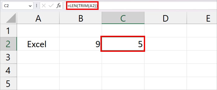
Now, the LEN will return 5 characters.
Example 6: Remove Space and Characters
If you have non-printing characters and excess spaces in values, you can nest the CLEAN function inside the TRIM function. This way, you’ll have both characters and spaces eliminated at once.
Here, we have the text string and character in C2. For this, use the given formula
=TRIM(CLEAN(C2))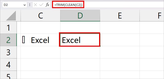
The formula will return Excel as a result.
Why is the Excel Trim Function Not Working?
As we mentioned earlier, you must enter the value inside the double quotation mark for text strings in the TRIM function. If you enter the formula like this =TRIM( Excel), it’ll only return #NAME? Error. To avoid such errors, use the quotation marks in the formula. Your formula should look like =TRIM(“ Excel”).
Having said that, do not use quotation marks for cell references in the TRIM function. Let’s say your value is in Cell A4. If you enter =TRIM(“A4”), you’ll get A4 in the cell. For cell references, you should enter =TRIM(A4) like we did in the above examples.