How to Transfer Data From One Excel Worksheet to Another

Transferring data between your worksheets can help organize your workbook— especially when you’re working on multiple worksheets.

Every time I want to derive a large set of data from another Excel Sheet, I use the advanced filter function to import the data. This streamlines my work, making it easier and saving me a lot of time.

There are multiple ways ranging from simple copy-pasting to using VBA code.

KEY TAKEAWAYS

• Use a simple copy-and-paste method to move data inside or outside your worksheet.
• Use the advanced filter option to extract specific data from a sheet with several columns.
• Lastly, using Power Query, you can link data to automatically update it whenever you make a change in the original sheet.

Using Copy and Paste Option

This option is similar to copying and pasting files or documents on your PC. It is an easy option when you want to transfer data between the same or different worksheets. Here’s how you can do it.

1. Open Excel.
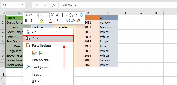
2. Go to the Excel Sheet and select the Cells which contain the data you want to copy.
   
3. Right-click and select Copy.
   
4. Now, go to the other sheet. Right-click on the cell where you want to add it and click Paste.
   

Use the Worksheet Reference

If you’re looking to transfer data from one worksheet to another, worksheet referencing is one of the many ways to transfer data from one Excel sheet to another. 

You need to use the = operator and click on the cell with the data you wish to reference—and the value will automatically appear on your worksheet.

1. Open the Excel sheet containing the data set.
   
2. Open a different sheet where you want the data to be copied. 
   
3. Type = on the cell where you want the data copied.
4. Open the Sheet with the data and click on the cell with the data and hit Enter.
   

Using VLOOKUP Function

A different approach to transferring data from one Excel worksheet to another is by using the VLOOKUP function in Excel. Basically, what this does is it takes the cell number from a given sheet as a reference to return the value from a different column.

Syntax: =VLOOKUP(lookup_value,table_array,column_index_num,[range_lookup])

• lookup_value: It indicates the item you want to search.
• table_array: It is the group of cells that contain the source data.
• column_index_num: It is the position of the column where the data will return if a match is found.
• range_lookup: It specifies if you want your VLOOKUP to find an approximate(True) or exact match(False).

Let me show this with an example.

1. Open Excel Sheet and select the empty cell where you want your data to be transferred. 
   
2. Type in = and search for the VLOOKUP function.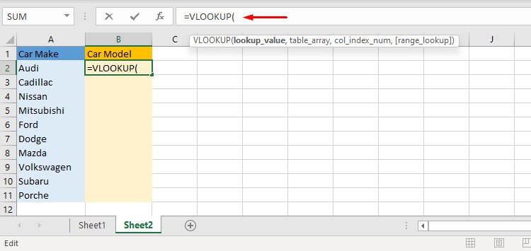
   
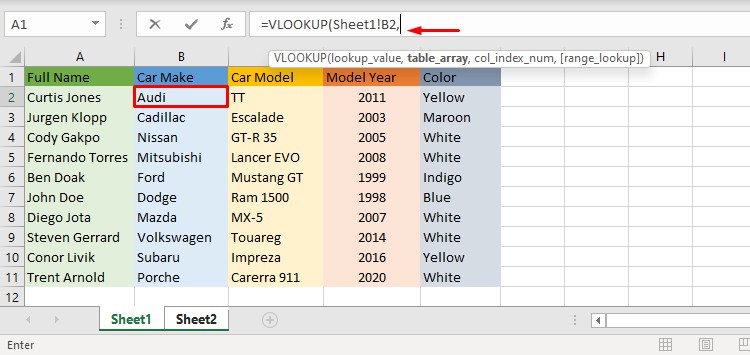
3. Go to the sheet which contains the data. 
4. Select the cell you want to copy and add a comma to the formula.
   
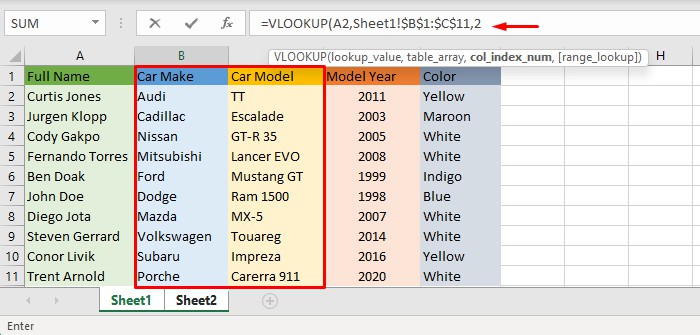
5. Select cells with data from Sheet 1 and press F4. 
   
6. Add a comma and write down which column contains the data. (Second column in this case)
   
7. Add a comma and type FALSE and close the bracket.  
   
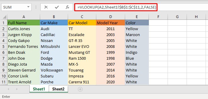
8. Press Enter to save changes and drag down to get all values.
   

Using the Advanced Filter

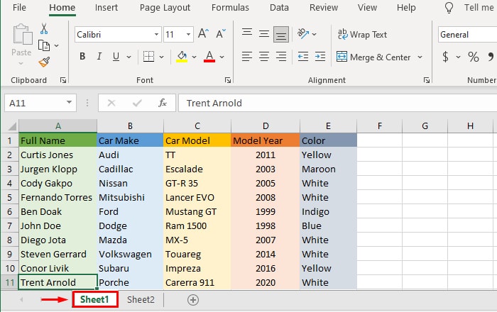
Let us suppose we have a list of data, and we only want to extract a specific section of data from that sheet. In such cases, we can use the advanced filter to transfer data based on our preset criteria. 

Here’s how you can use the advanced filter.

1. Open the Excel sheet containing your data. 
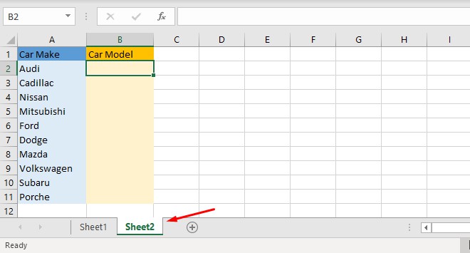
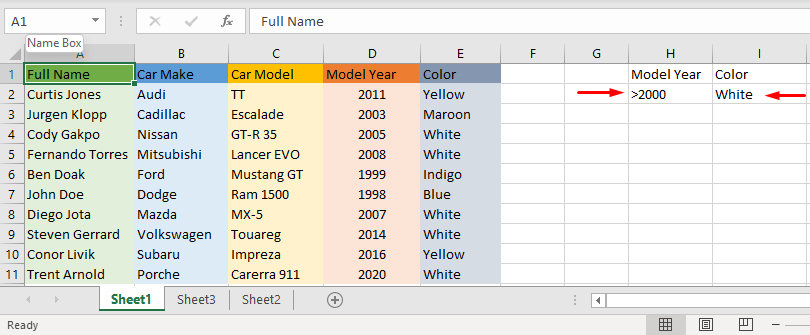
2. Alongside your data, create cells with exact same headings from your data. 
   
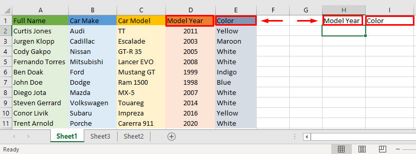
3. Beneath the column headings, put in your Criteria. 
   
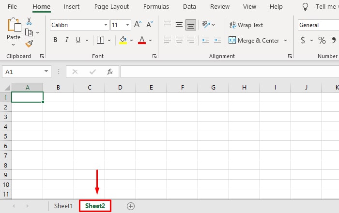
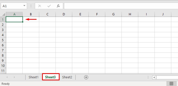
4. Open a new sheet and click on any cell where you want to transfer the data. 
   
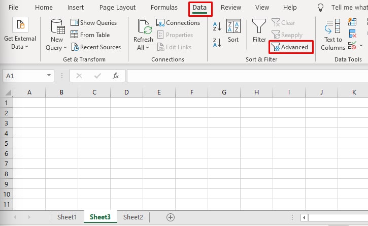
5. Click on the Data tab and select Advanced.
   
6. Go back to the original sheet and select your list range.
   
7. Select the Criteria range and select the column headings created in step 3.
   
8. Click on Copy to another location.
   
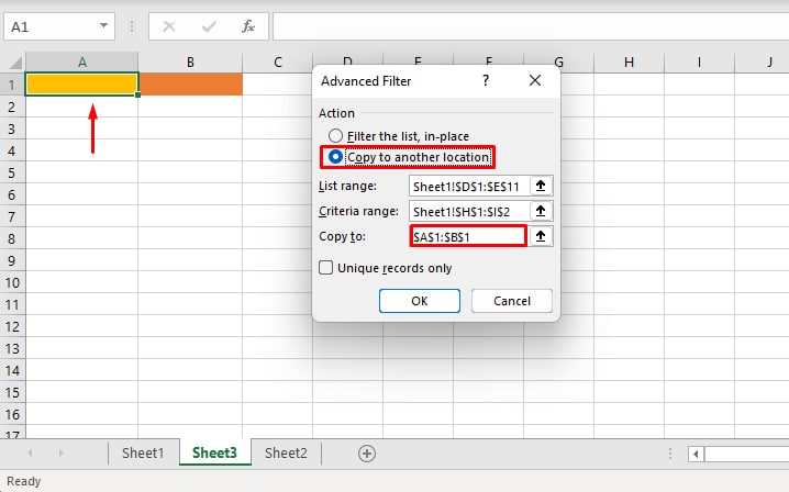
9. Click Copy to and select the cell where you want to transfer your data. 
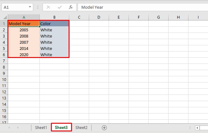
10. Click OK, and your filtered data will be transferred.
    

One major drawback of this method is that it does not automatically update data if you change your filter criteria.

However, you can get around this problem with the use of VBA code. 

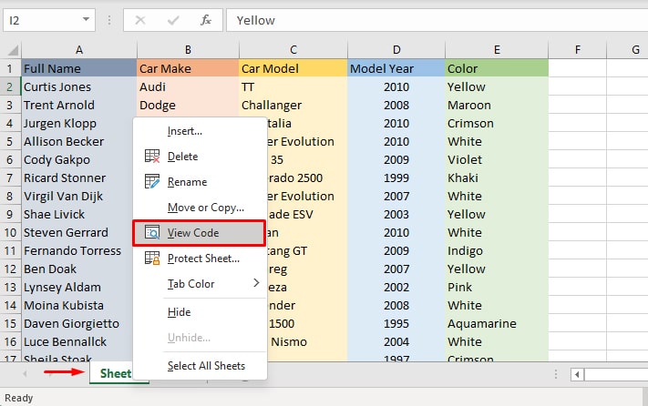
1. Open your Datasheet.
2. Right-click on the sheet tab containing your data and click View Code.
   
3. Copy the following code to your VBA with reference to your specific cell numbers.

Sheet2.Cells.Clear
Range("A1:E21").AdvancedFilter Action:=xlFilterCopy, CriteriaRange:=Range _
("H1:I2"), CopyToRange:=Sheet2.Range("A1"), Unique:=False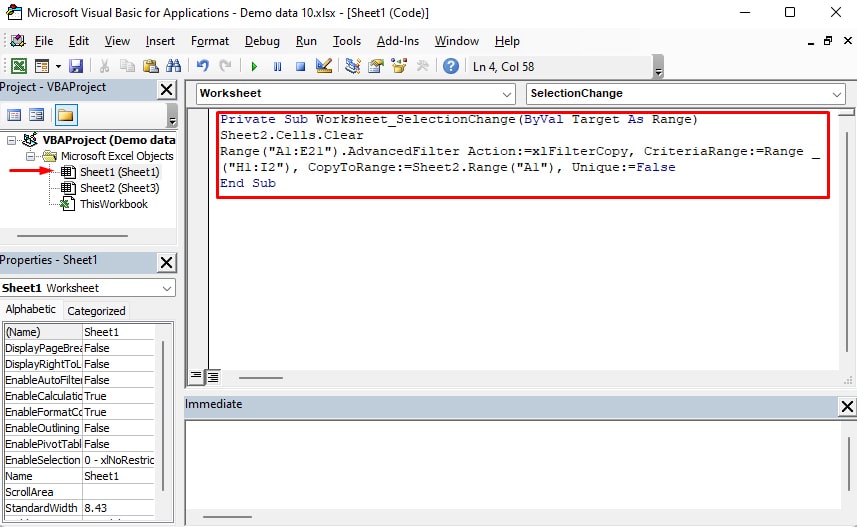

4. Close the VBA Editor.
5. Now the data on the new sheet will automatically update if you change the criteria in the original sheet. 
   

Using Power Query

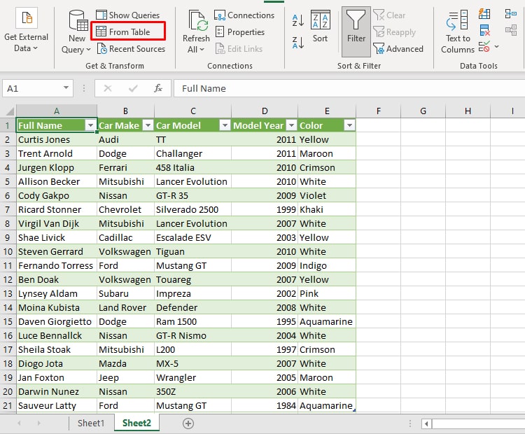
For this method, it is essential for your data to be in a table. Once your worksheet is in a table format, you can use the Excel Power Query tool to link your data across worksheets and update automatically. Here’re the steps.

1. Open your Datasheet.
2. Go to the Data ribbon.
   
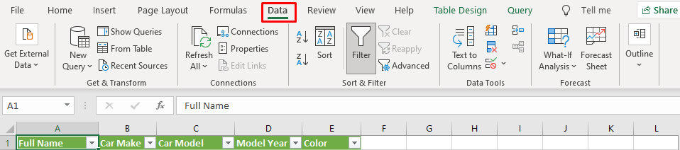
3. Make sure you’ve clicked somewhere on the table. 
4. Click on From Table, which will open the Power Query editor. 
   
5. Select the columns you want to work with. 
6. Click on Close & Load which will load the data in a new sheet. 
   

Now any changes you make on the original sheet will be updated to the new datasheet automatically. However, you will need to hit refresh on the new data sheet in order for it to be updated.