The TAKE function is a Lookup and Reference function in Excel that returns the specified number of rows and columns from an array. The TAKE function is comparatively new in Excel and many users have been taking a keen interest in its application.
Here’s a little dive through the TAKE function in Excel where we go into detail about everything including its arguments with examples.
Arguments Used in the TAKE Function
The TAKE function requires two arguments with one extra argument being optional. Here is the formula format for the TAKE function:
=TAKE(array, rows, [columns])- array: The array you wish to extract rows (and/or columns) from.*
- rows: The number of rows you are looking to extract.
- columns: The number of columns you are looking to extract.
The numbers you pass in the rows and columns section can be both positive and negative. If you enter a negative number, the TAKE function will return values from the end of the array.
Examples of TAKE Function
To simplify the explanation of the TAKE function, we have a few examples. In each example, we have used the same data set, only changing the values in the rows and columns section to show you what argument combination returns what value.
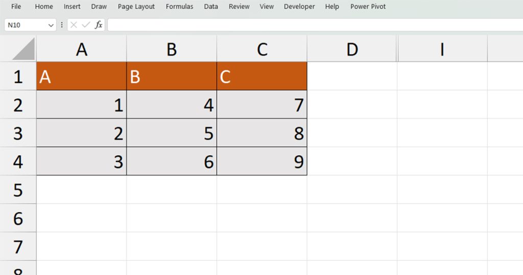
The data we will be using consists of three rows and three columns.
Example 1: Extract the First Two Rows
In this example, we will be using the TAKE function to return us the first two rows in the set array. For this purpose, we need to construct the TAKE function in the following formula:
=TAKE(A2:C4,2)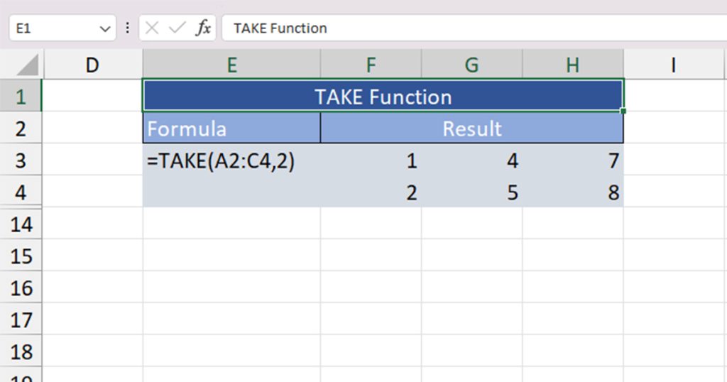
Example 2: Extract the First Two Columns
Using the TAKE function, you can also choose to return values in a column. For this, you will have to leave the section for rows empty and then enter the column value. Here is the formula we will be using to extract the first two columns:
=TAKE(A2:C4,,2)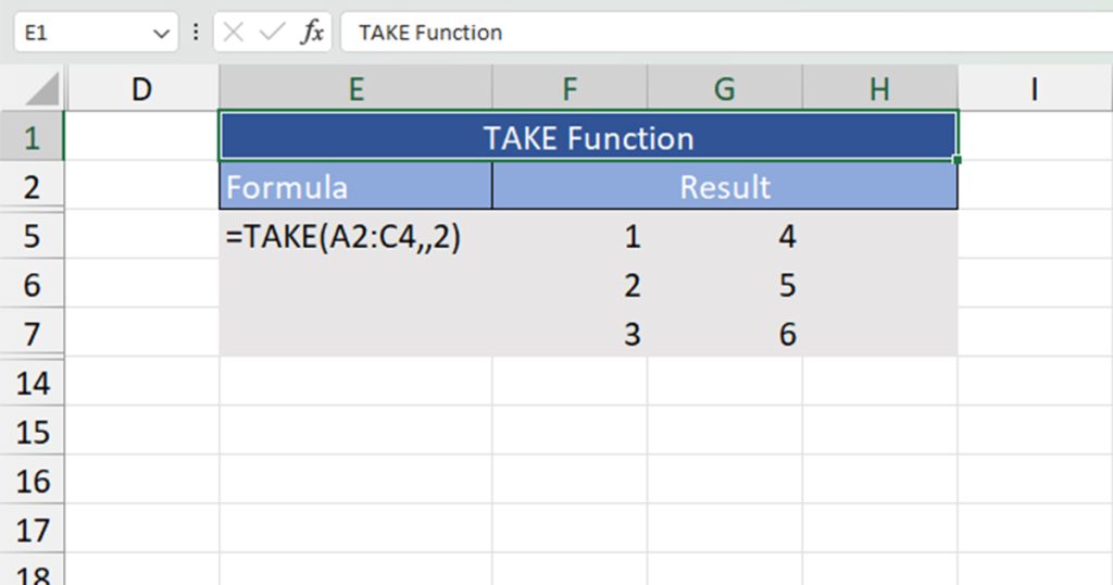
Example 3: Extract the Last Row
You can also extract from the last row using the TAKE function. Instead of using a positive value in the row section, swap it out with a negative value. Here is the formula we will be using to extract
=TAKE(A2:C4,-1)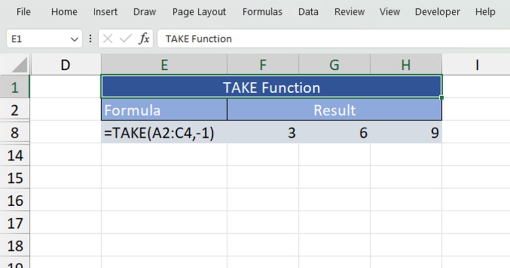
Example 4: Extract the Last Column
Similar to extracting rows from the bottom, you can also extract columns from the left using a negative value. Here’s the formula we used for the TAKE function to return the last column of an array:
=TAKE(A2:C4,,-1)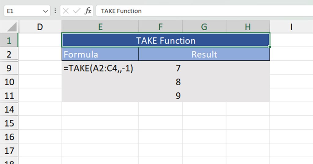
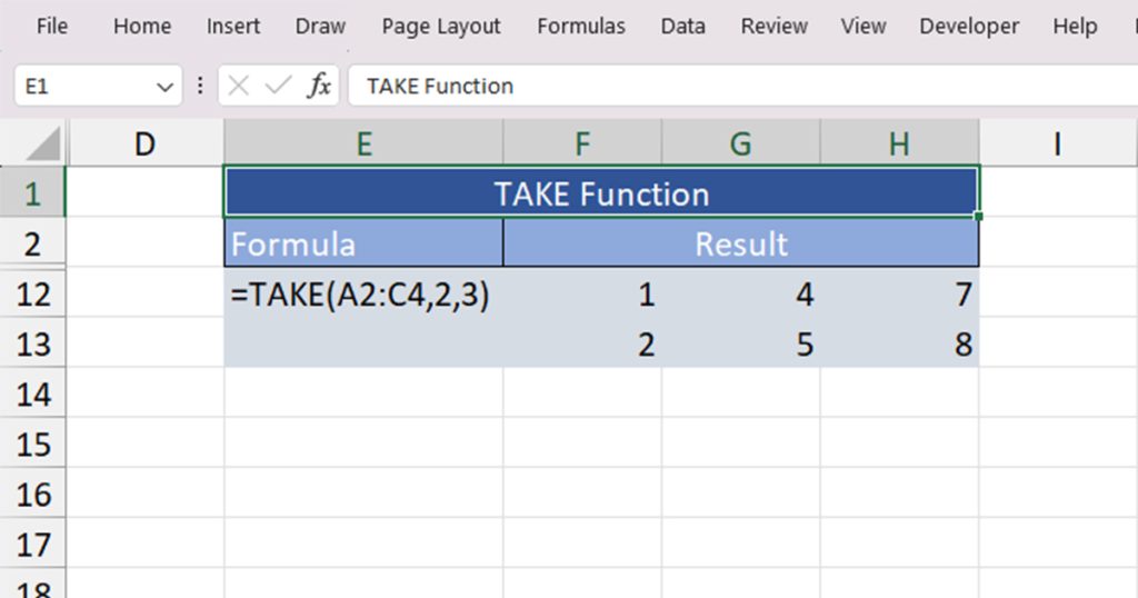
Example 5: Extract the Second Row from the Third Column
You can also use the TAKE function to return values by specifying both the row and column. For instance, if you return a value in the first row and first column, you will get the first value in the array. In this example, we will be extracting all values from the second row and the third column, which is also the last column.
Here is the formula we will be using for the TAKE function to return these values:
=TAKE(A2:C4,2,3)