Shortcut Key for Filter in Excel (7 Ways)

Filtering data is a lifesaver when you’re dealing with a vast data set. Filtering your data set makes it convenient for users to sort your data alphabetically, by color, or by the data itself. For instance, if you’re studying a sales sheet, you can filter out individuals that have already made the payment.

While you can access the Filter tool from the Data tab, you can also use a list of shortcuts to filter your content. In this article, we have included all the shortcuts you can use to filter your data in Excel.

Shortcuts to Filter Data in Excel

In this article, we have listed seven shortcuts you can use while filtering data from a range in Excel. 

Enable/Disable Filter

To create a filter, select the column header and use the following shortcut:

Ctrl + Shift + L

You can also use this shortcut to disable the filter.

Open Filter Options

After you’ve activated the filter tool in the data range, you can use the following shortcut to open the Filter menu:

Alt + down arrow

Move Between Filter Options in the Menu

To move between the options in the Filter menu, you can use the up and down arrow keys. The arrow keys will select these options, which you can then hit Enter to confirm.

Use the Underlined Letter to Perform a Task

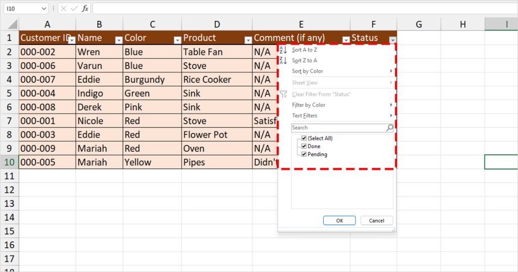
When you open the Filter menu, you can see that there’s a letter underlined in each option. These letters are underlined so that you can use these letters as shortcuts to perform the action. Here are the letters you can use once you have opened the Filter menu:

• S: Sort the filtered item in ascending order
• O: Sort filtered items in descending order.
• T: Sort filtered items by color.
• V: View the filtered range ina  Sheet view.
• C: Clear filter from the selected column.
• I: Filter data from range by color.
• F: Display text/number filter options to filter data range by

Enter Text in Search Bar

You can also filter the data range by entering the exact value on the search bar. For example, if you wish to filter out all data except “Confirmed”, you can deselect the Select All option, enter “Confirmed” in the search box, and select the box next to it.

Here is the shortcut you can use to enter such text in the search box:

Alt + down array + E

Reapply Filter

Once you activate the tool, your content is filtered out according to the criteria you set. The filter, however, does not work for the data you add after enabling the filter tool. To enable it for the data you add to the range later, you must use the following shortcut to reapply the filter:

Ctrl + Alt + L

Show All Items in Filtered Range

The Filter tool hides all rows that do not fit the set criteria in the range. In case you want to unhide these rows, select the column header you used to filter the range, then use the shortcut listed below:

Alt + down arrow + C

This will only clear the filter from the active column header.

Applying Filter Shortcuts in your Sheet

Now that we’ve gone through all the filter shortcuts, let’s see how these shortcuts work when dealing with data in Excel.

Here, we have a spreadsheet, tracking the orders of nine individuals. Firstly, let’s enable the filter tool.

1. Select any one of the six cells in row 1.
   
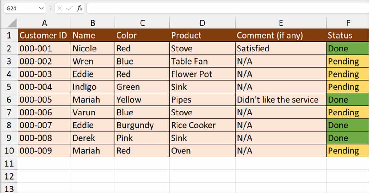
2. Use the shortcut to enable the filter shortcut,Ctrl + Shift + L
3. Select the column header with the range you wish to filter. We are going to filter the table according to column 6.
   
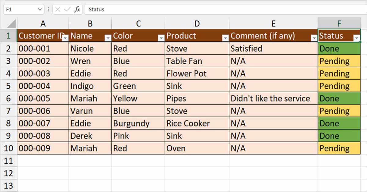
4. Open the Filter menu using the Alt + down arrow shortcut.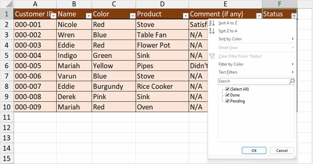
   
5. We can use the arrow keys to move between the options in the menu or select the option’s underlined letter.
6. For the sake of this example, let’s use this tool to show rows that have Pending in column 6. Use Alt + down arrow + E and enter Pending.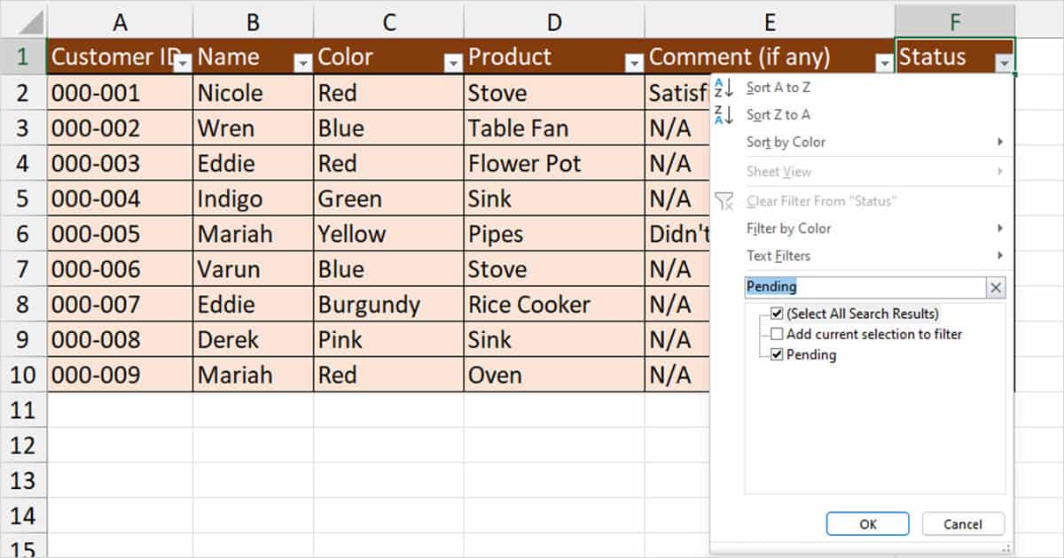
   
7. Hit Enter.
   
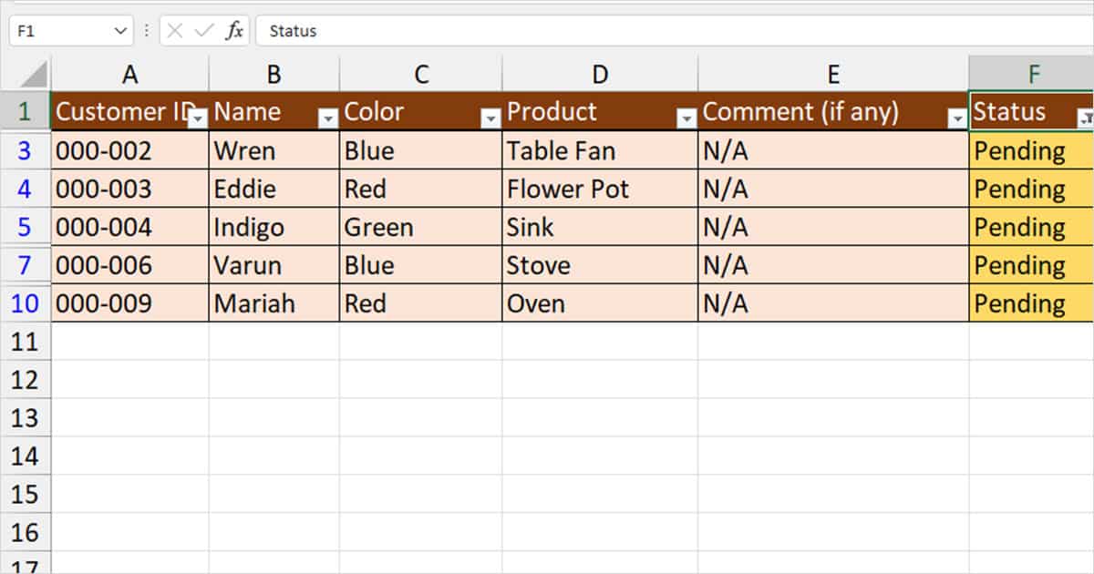
8. To show the hidden rows again, use Alt + down arrow + C.
9. If you wish to disable the Filter, select one of the column headers and use the Ctrl + Shift + L shortcut again.