If you’re creating a loan amortization schedule or allocating a personal budget, you might find the need to calculate the payment amount of a certain principal. For this, Excel has an amazing financial function called “PMT.”
While Excel users mostly opt for the PMT function to calculate the payment due on a loan, you could also use it to evaluate the savings amounts for future expenses. One of my favorite parts about using this function is you can create a payment calculator with it.
PMT Function Arguments
PMT function returns the payment amount for a loan in a fixed interest rate and period. The function arguments are:

=PMT(rate, nper, pv, [fv], [type])- Rate: Loan Interest Rate
- Nper: Number of Loan Payment
- Pv: Present Value or Principal amount
- [Fv]: Future Loan Value
- [Type]: Payment Due
- 0: Payment Due at End of Period
- 1: Payment Due at the Start of the Period
The PMT function arguments in the [] brackets are optional.
Examples of PMT Function in Excel
Example 1: PMT Function With Present Value
If you need to find out the payment due for loans, mortgages, timely credit card debts, etc., use the Present Value (PV) in the PMT function arguments.
Let’s say Amanda took a $25,000 personal loan from Jade with an annual interest rate of 5.7% for 3 years. Amanda wants to find out the payment amount on a different timely basis weekly, monthly, quarterly, semi-annual, and yearly so that she can estimate her budget.
To find out, first let us input the information in the cell below.
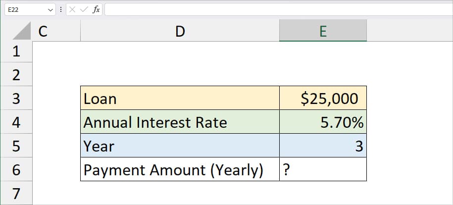
Since all of the information is in yearly annual, it’s pretty simple to calculate the annual payment amount.
For this, we will enter the formula as
=PMT(E4, E5, E3, 0)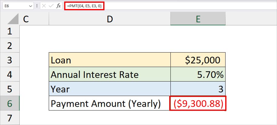
In the above formula, E4 is our annual interest rate, E5 nper, E3 principal amount. Since we have passed down 0 as a formula argument, it’ll calculate the payment due at the end of the period. The formula returned (9,300.88) in cell E3. So, Amanda needs to pay 9,300.88 amount yearly for the loan.
Now, let us find out the payment amount for different periods. Before you begin, quickly check out how we calculate the Rate and Nper value for each period first.
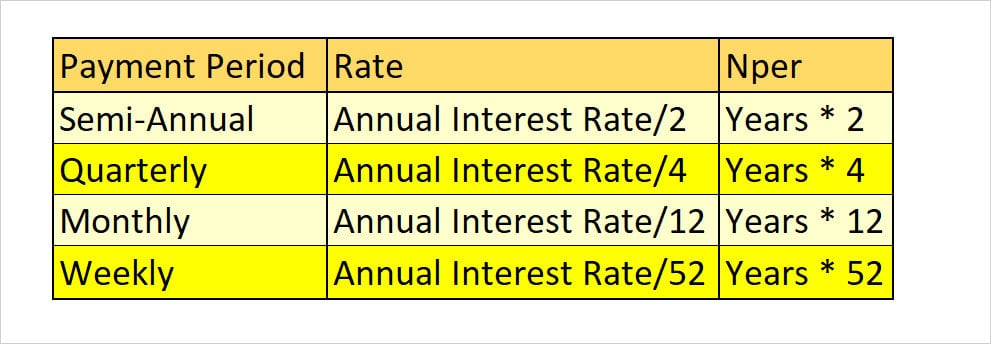
It’s solely up to you if you wish to calculate the nper and rate value before using the formula. But, here we will be calculating them in the PMT formula itself below.
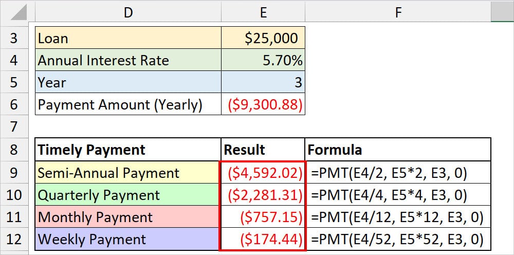
| Time Period | Formula | Result |
| Semi-Annual | =PMT(E4/2, E5*2, E3, 0) | ($4,592.02) |
| Quarterly | =PMT(E4/4, E5*4, E3, 0) | ($2,281.31) |
| Monthly | =PMT(E4/12, E5*12, E3, 0) | ($757.15) |
| Weekly | =PMT(E4/52, E5*52, E3, 0) | ($174.44) |
Example 2: PMT With Future Value
You can also use the PMT function to calculate the payment of future value (FV). I use the PMT function with the FV argument whenever I want to allot a sum of money in my savings account for upcoming expenses or events.
Suppose, I want to save money for a family vacation which is four years from now. The vacation will cost me around $10500. The annual interest rate for savings is 1.8%. I want to find out how much money should I allocate semi-annually (every 6 months) to save a total of $10,500.
For this, I’ll first input this information in the cell value. Then, to calculate, I will enter the PMT function as
=PMT(B3/2, B4*2, 0, B2)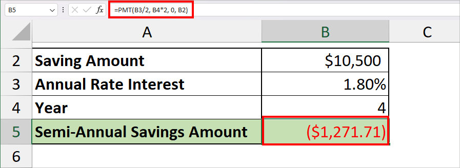
In the formula, I have entered 0 as the Present value. So, the formula resulted in ($1,271.71). This means that I need to accumulate that amount semi-annually for four years to save $10,500 for family vacations.
Create a Payment Calculator Using the PMT Function
We’ve covered the examples of using the PMT function above. But, did you know that you could also create a PMT calculator?
PMT calculator is especially helpful if you find yourself calculating the Loan Payment more often. This way you wouldn’t have to keep using the PMT formula and calculate everything from scratch.
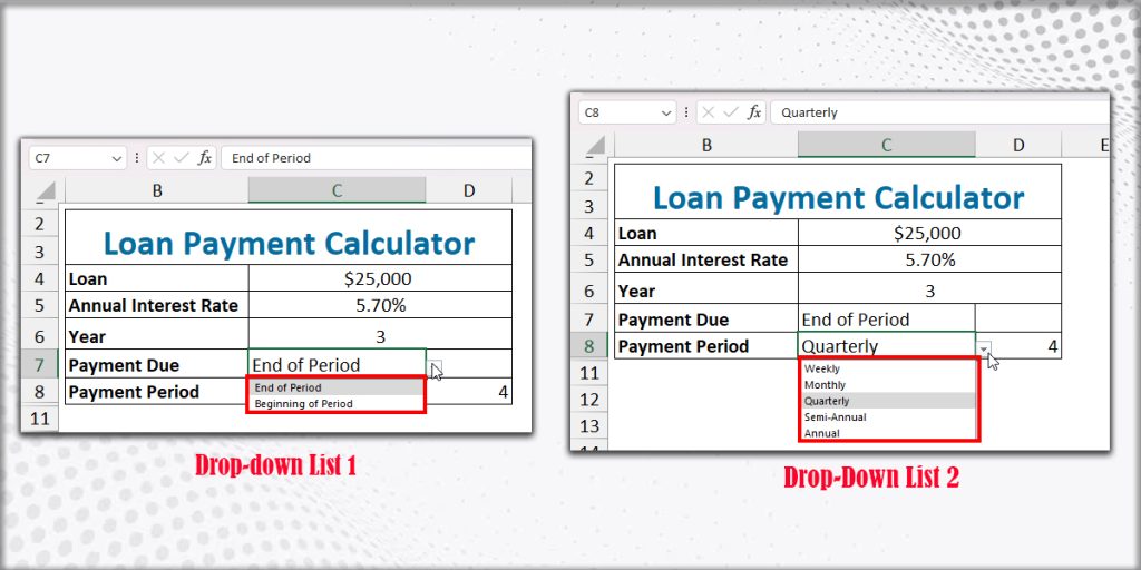
Step 1: Add Drop-down List
Here, we will add two drop-down lists for the Payment Due and Payment Period.
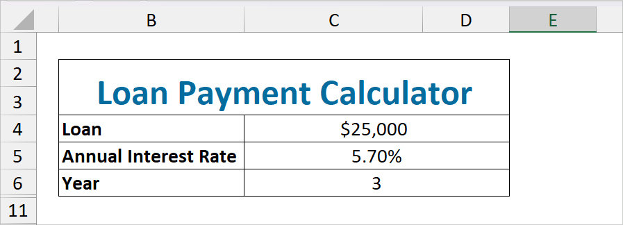
- Firstly, enter all the information in cells(Loan, Year, Interest Rate).
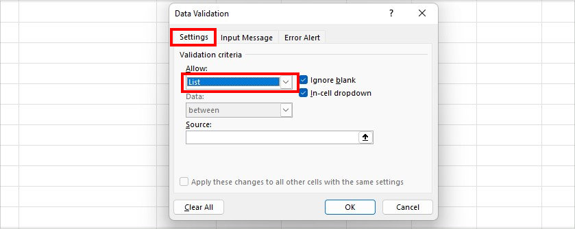
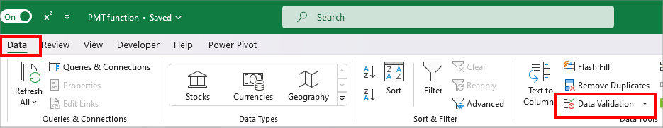
- Now, enter Payment Due in a new cell. Then, select the cell next to it. Navigate to Data Tab > Data Validation.

- On the Data Validation window, expand the drop-down for Allow and choose List.
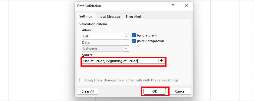
- On Source, enter End of Period, Beginning of Period and hit OK.
- Again, enter the Payment Period in another cell. Select a cell next to it and insert a drop-down list. From the Data Tab, click Data Validation.
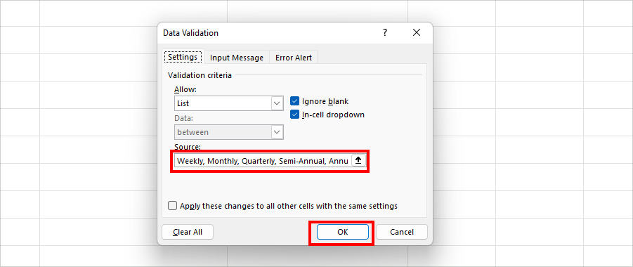
- On the window, stay on the Settings tab. Pick List for the Allow menu.

- Then, type in Weekly, Monthly, Quarterly, and Semi-Annual in the Source field. Click OK.
Step 2: Create a Lookup Table
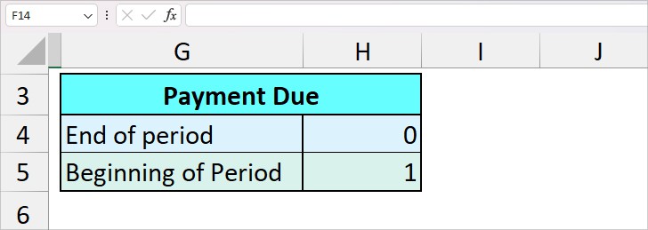
Firstly, let us create a Lookup Table for the Payment Due. Enter a heading in the new cell. Then, enter the Payment Due type in the cells like in the given picture. My lookup table is from G4:H5.
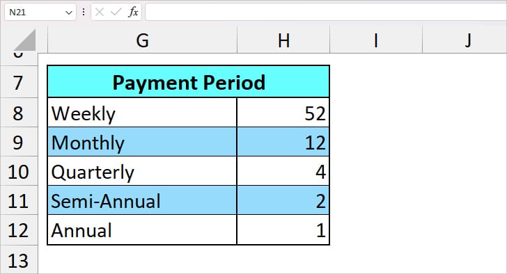
Now, insert the lookup table of the Payment Period heading. Here, I have entered the Period name and the time period in numbers. My lookup table is from G8:H12.
Step 3: Calculate Payment Due and Payment Period
To return the value of periods and payments due, let us use the VLOOKUP and IFERROR functions nested together. As an example, I will return end of the period and Quarterly.
| Find | Formula | Result | Description |
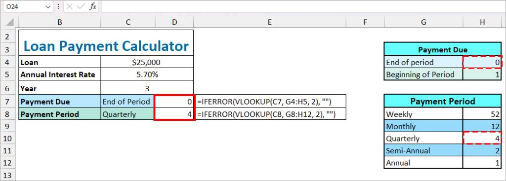
| Payment Due (End of Period) | =IFERROR(VLOOKUP(C7, G4:H5, 2), “”) | 0 | VLOOKUP function returns the value of the End of Period from the second column of a lookup table. In case there is no value, the IFERROR function will return a null. |
| Payment Period (Quarterly) | =IFERROR(VLOOKUP(C8, G8:H12, 2), “”) | 4 | In this formula, the VLOOKUP function returns the Quarterly Payment period from the lookup table. Since we’ve passed down IFERROR function, the formula would return null if the lookup value was not found. |
Step 4: Calculate Payment Using PMT
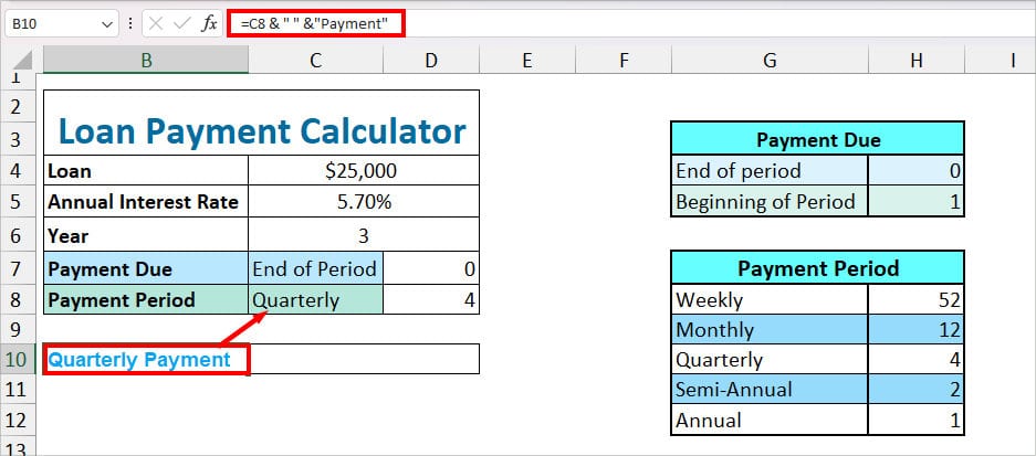
Finally, in this step, I will calculate the PMT. But, before that, I will enter =C8 & " " &"Payment" in cell B10 to link it with the Payment Period cell. I did this to make the heading in cell B10 dynamic.
Now, to calculate Quarterly Payment, I will enter the PMT formula.
=IFERROR(-PMT(C5/D8, C6*D8, C4, D7), "")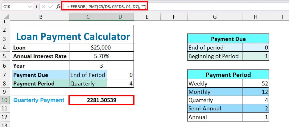
The formula returned 2281.30539. In the formula, we’ve entered the – (minus) sign before the PMT formula to return the value in a positive number.
Now, whenever you choose a different Payment Period in the drop-down list, you’ll automatically have that value.
Avoid These Errors in the PMT Function
| Cell Error | Possible Causes |
| #NUM! error | When you’ve entered a negative number in the rate argument. When the value of nper = 0. |
| #VALUE! error | If you’ve passed down more than one text argument in the formula. |