VLOOKUP pushes the envelope when used on a lookup table. With this, you can look for and retrieve data, check for accuracy, merge data, create automatic reports, and much more. However, this functionality of VLOOKUP ends up being quite limited on a PivotTable.
The PivotTable summarizes a large data table in to manageable and interactive layout. So, instead of using ranges, it creates fields of data. VLOOKUP takes cells and cell ranges as references from a data table. This functionality, unfortunately, is not supported by Pivot Tables.
While you can still use VLOOKUP on a PivotTable, I would highly suggest you look into the GETPIVOTDATA() function in Excel. The function is quite similar to VLOOKUP but takes in row and column references instead of cells. In this article, I will go into detail about using VLOOKUP in a PivotTable, and also discuss its limitations.
VLOOKUP on PivotTable
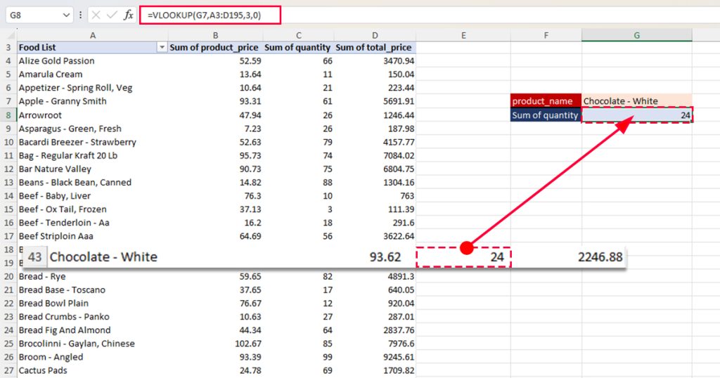
Take a look at this Pivot Table. Here, we have a list of all food items purchased by a catering company.
Let’s use VLOOKUP to look up the total number of White chocolates purchased by the company. We created a little table on range F7:G8 to help look up our value. Here is how we will be constructing our formula using the VLOOKUP function:
=VLOOKUP(G7,A3:D195,3,0)
Why NOT to Use VLOOKUP on a PivoTable in Excel
You may be thinking, “Hey, I thought you said VLOOKUP does not work on PivotTables!”. Well, it’s a mix of yes and no. You may be thinking that VLOOKUP just worked on our PivotTable, but it actually only reflected the value that is currently on the cell.
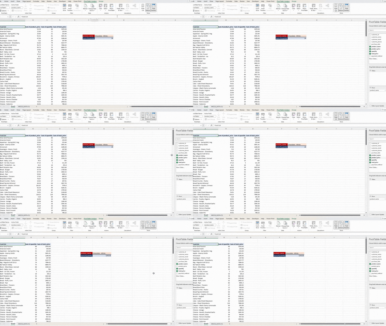
PivotTables use fields that are made up of the rows and columns of your source data table. You can switch what fields you wish to see as what values are in the field list. In our PivotTable, we have currently selected the fields for product_name, product_price, quantity, and total_price.
Let’s see what happens when we switch out one of these fields from the PivotTable.

Oops! According to VLOOKUP, the total quantity purchased for Chocolate-White is now 2246.88. Investigating the formula, we see that VLOOKUP is still referencing the value in the third column, adjacent to Chocolate – White. When we switched out the field for the product_price, the Sum of total_price became our third column.
What to Use Instead of VLOOKUP in a PivotTable
Now that we’ve established that VLOOKUP does not extract values from a PivotTable but simply the cell location, here comes the real question: What can you use instead of VLOOKUP on a Pivot Table? Well, you can use GETPIVOTDATA instead of VLOOKUP!
What is GETPIVOTDATA?
GETPIVOTDATA is a lookup function in Excel, that extracts value from a PivotTable by taking the field name and item as a reference. In contrast to VLOOKUP, GETPIVOTDATA does not take cell locations as a reference.
Here is the syntax GETPIVOTDATA follows when constructing a formula:
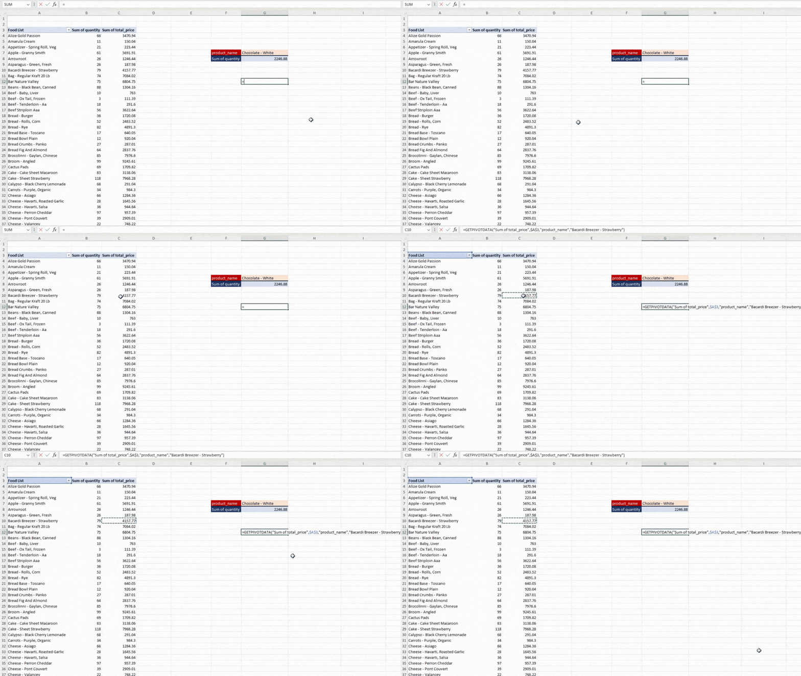
=GETPIVOTDATA(data_field, pivot_table, [field_1,item_1], [field_2,item_2],...)Here’s something interesting about PivotTables. When you enter the equals to operator (=) and click on any location inside your spreadsheet, you’d expect to see the cell location. This is not the case when it comes to PivotTables.

When I clicked on the cell C10 of a PivotTable, I got =GETPIVOTDATA("Sum of total_price",$A$3,"product_name","Bacardi Breezer - Strawberry") instead of the typical =D10 reference.
This is the value of your data field. As we discussed before, PivotTable does not hold its data in cells, therefore, it does not return a cell reference. Now that we know what the role of GETPIVOTDATA is, let’s build a formula to look up our values on a PivotTable.
How to Use GETPIVOTDATA on a PivotTable
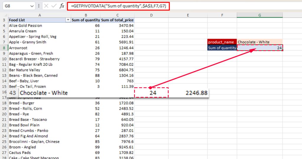
Firstly, you will need to specify the data field, and the name of your pivot table to get a value. Then, you have to enter the field name and item that holds the data you wish to look up. Let’s use the same example and check the quantity of Chocolate – White in our PivotTable using GETPIVOT.
Here’s the formula we will be using:
=GETPIVOTDATA("Sum of quantity",$A$3,F7,G7)
Let’s break down the arguments used in this function:
| Syntax | Argument | Returns | Description |
| data_field | “Sum of quantity” | Sum of quantity | As our data is in the “Sum of quantity” field, this will be our reference for data_field. Do not use a cell reference for this argument as it will return the #REF error. |
| pivot_table | $A$3 | Food List | The name of your PivotTable. This is usually the column header of the first column. |
| [field_1 | F7 | product_name | The name of the field your item is in |
| item_1] | G7 | Chocolate – White | The name of the item |