OFFSET is a part of Excel’s lookup and reference functions. While this function has been around for quite a while, Excel made a significant improvement in this function after version 2019. This update allowed OFFSET to return an array instead of only a singular value.
This improvement could have you wondering how you can use OFFSET to return an array. Whether you’re a beginner looking to learn more about this powerful lookup function, or a veteran updating yourself, allow this article to give you a brief overview of the OFFSET function and its application.
What is OFFSET?
If you’re a beginner looking to learn more about the functions in Excel, you could be interested in getting a brief description of OFFSET before getting into the technicals.
OFFSET is a lookup function. It uses the reference you’ve set and navigates to a cell using the coordinates you’ve set as the row and column.
For example, your reference point is in A1. You want the OFFSET function to return you a value in cell B3. Your coordinates will be (2,1) because B3 is two rows below, and one column to the right of your reference point, B3.
The application of OFFSET is diverse. You can use OFFSET simply as a lookup function, or you can nest them in other functions like SUM and AVERAGE. We will discuss more about its application under the examples section in this article.
Arguments Used in OFFSET
Lookup functions usually have longer arguments inside their parameters. This, sometimes may look intimidating, but I assure you it’s nothing complicated.
OFFSET has five arguments in total; out of which, three are required and two are optional. Here’s how the OFFSET function is written as a formula including its arguments:
=OFFSET(reference, row, column, [height],[width])- reference: This will be your reference point. Any value you insert next will be with respect to this cell location.
- row: The number of rows the value you wish to return exists in. If your value is above the reference point, enter your number in negative. If it’s above, use a positive value.
- column: The number of columns you wish to return exists in. If your value is to the left of the reference point, enter your number in negative. If it’s on the right, use a positive value.
- [height]: If you’re looking to pass an array, select how many rows you wish to return from the destination point.
- [width]: If you’re looking to pass an array, select how many columns you wish to return from the destination point.
Application of OFFSET in Excel
There are three distinct ways you can use OFFSET in Excel. You can use OFFSET to return a singular value, an array, or nest it inside other functions in Excel. In this section, I have used all three methods in easy-to-follow examples.
Example 1: Use OFFSET to Lookup a Singular Value
When you use OFFSET to look up a singular value, you don’t have to enter the values for height and width, the optional values.
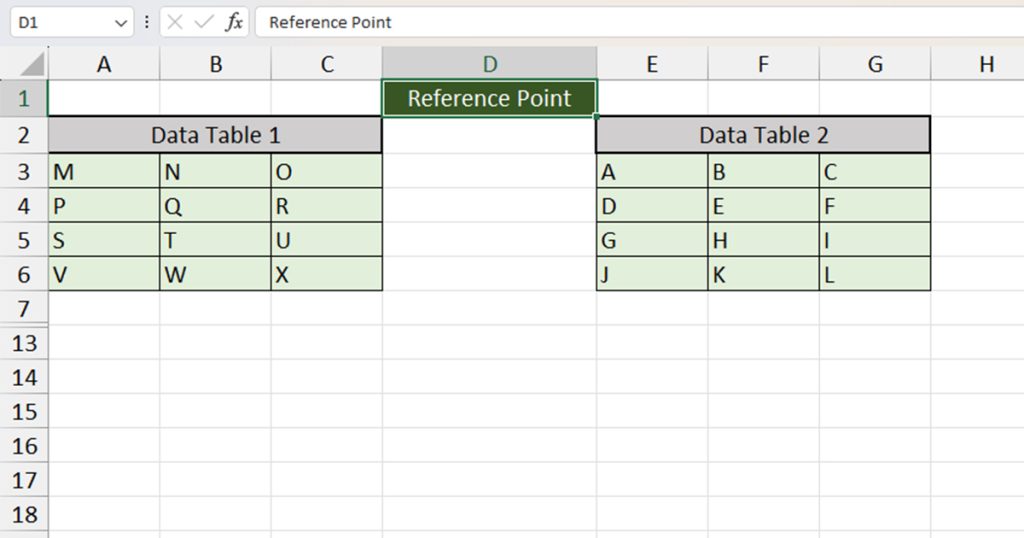
Take a look at this spreadsheet. I’ve set cell D1 as our reference point. There are two data tables in this sheet. One value exists in the range A3:C6 and the second in E3:G6. Any value we enter in the row and column section of the arguments in OFFSET will be with respect to D1.
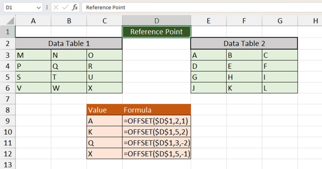
Let’s use OFFSET to return Q and X from the first data table, and A and K from the second data table.
| Value | Formula | Description |
| A | =OFFSET($D$1,2,1) | “A” is in cell E3. Cell E3 is 2 rows below and one column to the left of D1. |
| K | =OFFSET($D$1,5,2) | “K” is in cell F6. Cell F6 is 5 rows below and two columns to the left of D1. |
| Q | =OFFSET($D$1,3,-2) | “Q” is in cell B4. B4 is 3 rows below and two columns to the right of D1. |
| X | =OFFSET($D$1,5,-1) | “X” is in cell C6. C6 is 5 rows below and 1 column to the right of D1. |
Example 2: Use OFFSET to Lookup an Array
You can only use this method if you’re currently using Excel version 2019 or above. There isn’t a way for OFFSET to return an array if you’re using the earlier versions.
When you’re using OFFSET to return an array, you will have to specify the height and width of the array. OFFSET will return your array depending on this value. For example, if your value for height and width is (2,2), OFFSET will return an array that is two rows and two columns below the destination cell.
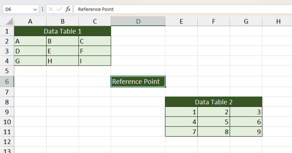
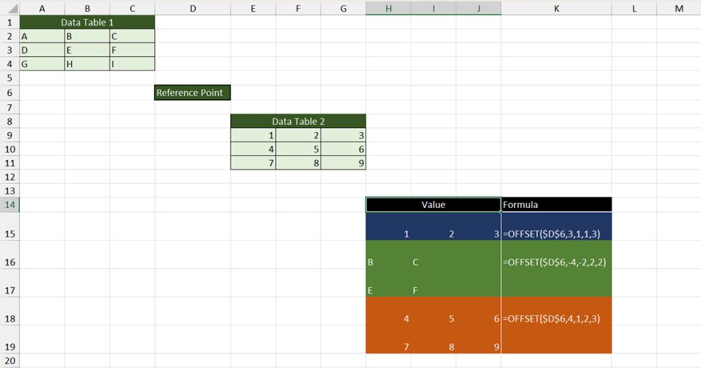
Here is another spreadsheet with two data tables. The first table is in A2:C4, while the second one is in E9:G11. Our reference point is in the middle, in cell D6. Let’s use OFFSET to extract arrays from both of these data tables.
| Value | Formula | Description |
| 1 2 3 | =OFFSET($D$6,3,1,1,3) | The destination cell is E9. OFFSET extracts values from three columns on the right in the same row as E9. |
| B C E F | =OFFSET($D$6,-4,-2,2,2) | The destination cell is B2. OFFSET extracts values from two columns on the right, and two rows below B2. |
| 4 5 6 7 8 9 | =OFFSET($D$6,4,1,2,3) | The destination cell is E10. OFFSET extracts values from two columns on the right, and three rows below E10. |
Example 3: Nesting OFFSET Inside Other Functions
Before OFFSET returned an array, the only way to use OFFSET as an array function was by nesting it inside another function that supported array values.
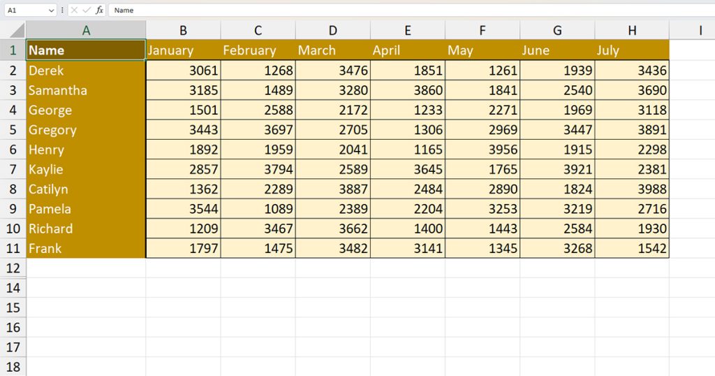
In this table, I have prepared a mock annual finance sheet of a company. Let’s say our manager asked us to prepare a dynamic formula to calculate the sales of the company in the last three months. This means, every time you add a new month, the formula should automatically update itself.
We will be nesting OFFSET inside the SUM function to create this formula. Inside OFFSET, we will have to use the COUNTA function to make this formula. Here is the formula we used for this data table:
=SUM(OFFSET(B1,1,COUNTA(B2:M2)-3,10,3))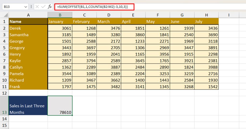
We know the formula is a bit long. So, there’s a little evaluation of the formula to see which part results in what value.
| Formula | Result | Description |
COUNTA(B2:M2) | 7 | Counts the non-empty cell in the range B2:M2. For our table, the result is 7. |
OFFSET(B1,1,COUNTA(B2:M2)-3,10,3) | F2:H11 | OFFSET uses a cell below 1 row, and 4 (7-3) column to the right of B1 as the destination cell. Then, it returns an array of 10 rows in height and 3 columns in width. |
SUM(OFFSET(B1,1,COUNTA(B2:M2)-3,10,3)) | 78610 | The sum of F2:H11 is 78610 |