Excel has a number of functions you can use to retrieve values from a data range. This is so you can save the time you would normally spend while scrolling through the sea of information to fetch data.
While analyzing a bigger data set, I like to sometimes use the LOOKUP function, or even nest the INDIRECT and COUNTA functions to create a lookup formula. In some cases, you could even use one of Excel’s navigation shortcuts to land yourself in the last value of the data range.
Use Excel Shortcut
Shortcuts in Excel help most with productivity. Although this method will not exactly paste the last value of your column in the selected cell, I think it’s the quickest way to get to the last value of a column.
Simply, select any cell you wish to retrieve the last value of. Then, use the Ctrl + down arrow keys to land on the last, non-empty cell of the column. I think is the most hassle-free method as it involves no use of functions. Additionally, the navigation is instantaneous, saving you a lot more time.
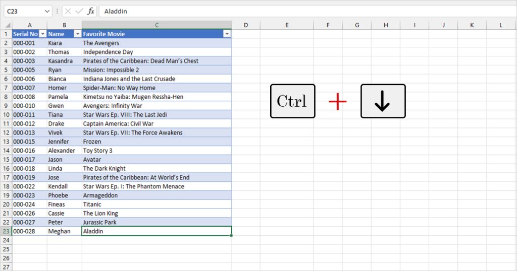
The only downside of this method is that you’ll have to keep using the shortcut to view the end value. This is still a pretty good option if you’re looking for a quick view of your data.
Nest INDIRECT and COUNTA Functions
If you’re looking for a more dynamic method, you should nest the INDIRECT and COUNTA functions. Pairing these functions creates a formula that will retrieve the last value of the set column in Excel. When you use this method, any value, even if it’s an error is retrieved from the column.
The only downside to this method is if your column has blank cells in between them. This is because the COUNTA function only counts non-empty cells. You can use the formula in the following format:
=INDIRECT(“column alphabet”& COUNTA(range))
To better explain this formula, let’s look at this example. In this spreadsheet, we have 11 values, including the header. Using our formula, we’ll be extracting the last value from the column, which is “Reggie Brown”.
In cell C1, we entered the following formula:
=INDIRECT("A"&(COUNTA(A:A)))
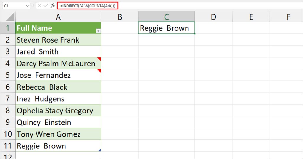
The COUNTA function will count all the instances where the cells are non-empty. This will return 11. This will return us A11 as we have passed the column letter, A as a text argument. “A11” will be used as a reference for the INDIRECT function, which will then extract the contents of the cell location.
Use the LOOKUP Function
If you think your range has a blank space in between, you should use the LOOKUP function to extract the last value. This function works for all cell content except for errors. Therefore, if your last value is an error, the LOOKUP function will ignore the cell. You can use the method with the INDIRECT and COUNTA functions if you think the last could be an error.
Use the LOOKUP function in the following formula format:
=LOOKUP(2,1/(range<> “”),range)
In this spreadsheet, we have 12 values including the table header. There is an empty cell in the second last value. We will be using the LOOKUP function to extract the last value, “Reggie Brown”.
In cell C2, we use the LOOKUP function in the following formula:
=LOOKUP(2,1/(A:A<>""),A:A)
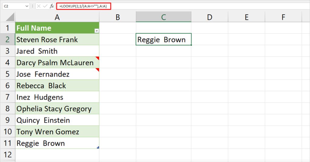
Here’s a bit of the formula. We passed 2 as our lookup_range, 1/(A:A<> “”), as our lookup_vector, and A:A as our result_vector.
- (A:A<> “”): The lookup vector is a condition to know if the cell is empty or not. The function will run through all cells in column A and return TRUE or FALSE depending on if the cell is empty or not. In our case, all cells except cell 11 will return TRUE, as they are not empty.
- 1/(A:A<> “”): In programming, TRUE returns 1 while FALSE returns 0. In the next phase of our function, this information comes to use. If the cell is nonempty, this part of the formula will return 1/1 = 1. However, if it is empty, it returns 1/0 = DIV/0! error.
- LOOKUP(2,1/(A:A<> “”),A:A): The LOOKUP function will look for the cell returning 1. However, that does not exist. So, the function will return the value it assumes is closest to 2; the last cell that returns 1. Therefore, the LOOKUP function will return the last nonempty cell value of column A, Reggie Brown.