How to Insert Arrow in Excel

Arrows can be very helpful to make your readers understand your data analysis at glance. In Excel, you can add three different types of Arrows. Depending on the arrow you use, you could showcase the relationships, portray trends, outline formulas, and many more. 

To illustrate Excel charts, basic arrow shapes or symbols would do the work. But, if you are delivering a report, use Trend arrows as a graphical representation to indicate the changes in value. Similarly, to check formulas in your spreadsheet, you can insert trace dependents or trace precedents. 

Insert Arrow Symbol/Shapes

If you are a beginner in Excel, you can start with simple arrow symbols, shapes, SmartArt, etc. You can use them to point out cell values or display relationships. Depending on your need, check out these methods.

From Symbol

1. Go to Insert Tab.
2. Click on Symbol.
   
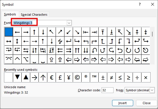
3. On the Symbols box, select Wingdings 3 on Font menu.
   
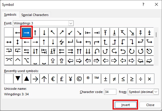
4. Pick an Arrow and choose Insert.
   

From Shapes

1. On your spreadsheet, navigate to Insert Tab.
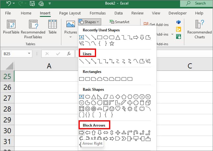
2. On the Illustrations menu, click on Shapes. 
   
3. Choose an arrow from the Lines and Block Arrows menu. Here, we have taken a Right block arrow.
   
4. Now, draw an Arrow in the cell range. 
   
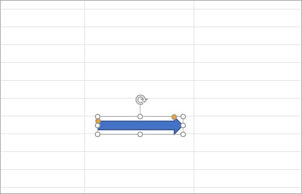
5. To format the arrow, click on the Shape and go to Shape Format Tab.
   
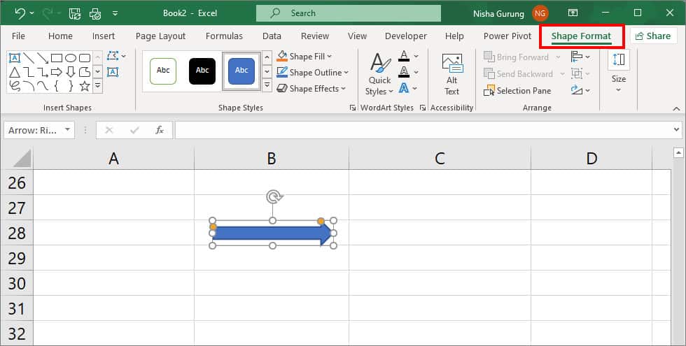
6. You can edit Shape Styles, Sizes, Arrange, Add Text, change Outlines, etc.

From SmartArt  

1. On your worksheet, click on Insert Tab.
2. Click SmartArt in the Illustrations menu. 
   
3. Now, you can go through several menus on the right panel to browse Arrow designs. Pick any one SmartArt Arrows and hit OK button. 
   
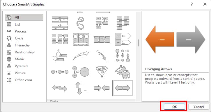
4. You can format the SmartArt Arrows as per your wish. 
   

Using Wingdings 3 Font

1. Open your Excel worksheet.
2. Click on the Cell you want to add arrows.
3. Enter these characters (!, ", #, $)  respectively in the cell as in the given picture.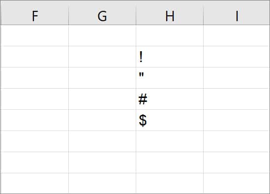 
   
4. Now, navigate to the Home tab. On the Font menu, set the font to Wingdings 3.
   
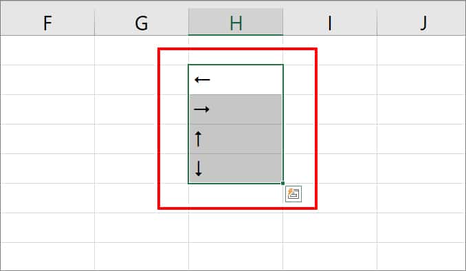
5. The characters will change into Left, Right, Up, and Down arrows. You can copy and paste the arrow or use the auto-fill handle to insert them into other cells.
   

Insert Trend Arrow

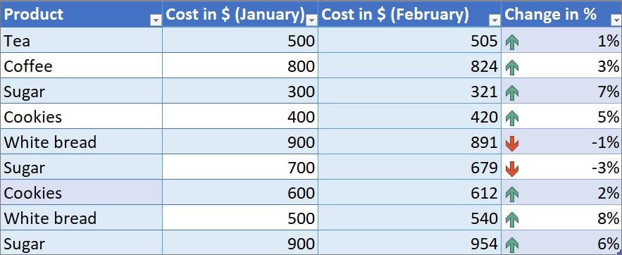
Trend Arrows can be used to represent the positive or negative changes in the current value. For Instance, a simple green upward arrow would indicate the value as an increased trend. Similarly, the red down arrow as a decreased trend. 

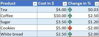
Adding a trend arrow is a little complex compared to basic arrow shapes. However, we have provided two easy methods to insert them which are beginner-friendly.

From Format Cells

In this approach, we will create a custom format by copying and pasting the arrow symbols to the number format. You can also add colour to the arrow as per your preference to showcase the trend. 

1. Launch Excel and open your worksheet.
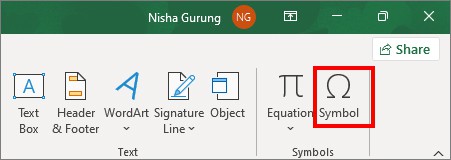
2. Click on an Empty cell. Then, go to Insert Tab > Symbol.
   
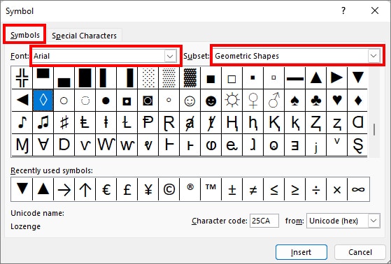
3. On the Symbols tab, set the Font to Arial. Then, choose Geometric Shapes for the Subset menu. 
   
4. Select the Up arrow and click on Insert to confirm. Again, double-click on Down arrow to add it.
   
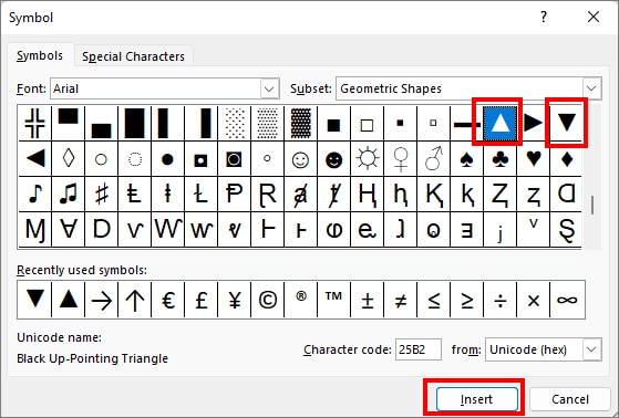
5. Once done, Copy both arrows. 
   
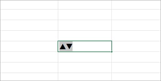
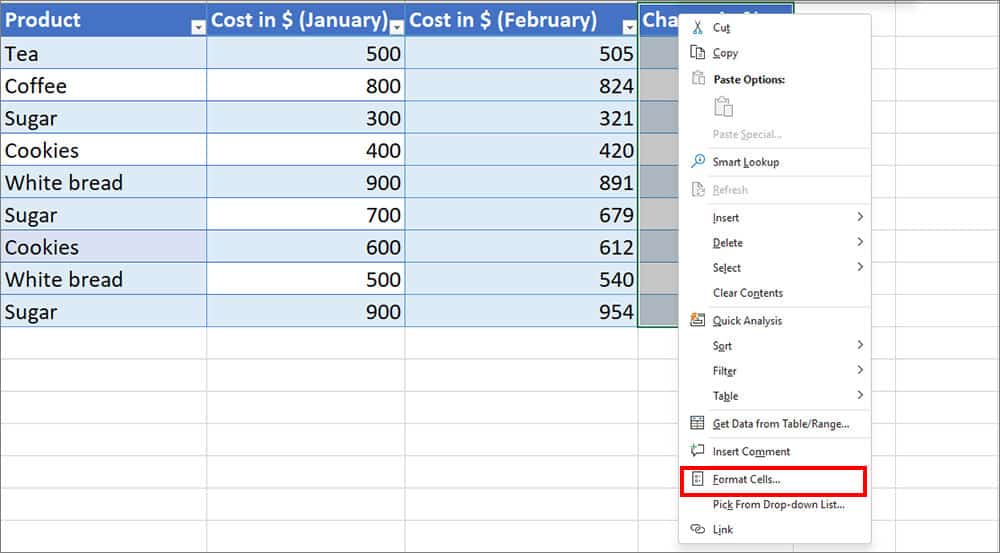
6. Now, highlight the Cell ranges with data and right-click on it. Click on Format Cells. 
   
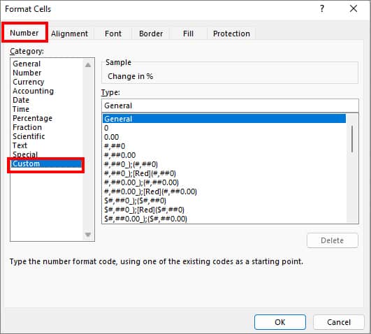
7. On the Number tab, go to the Custom menu on the right panel.
   
8. Under Type, Paste both Arrows in the field. The format should be like this, ▲0%;▼0%.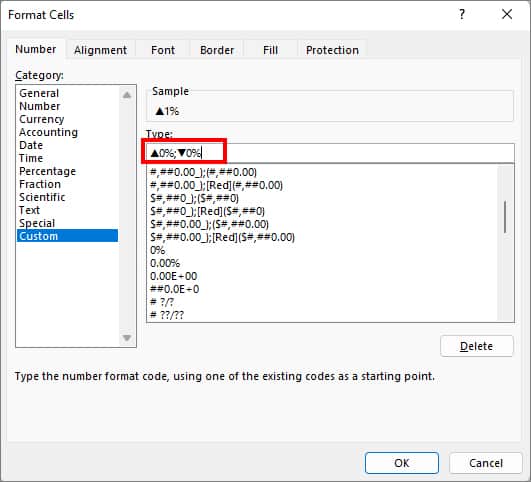
   
9. It will add Up and Down arrows on your data.
   
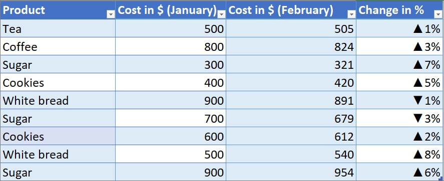
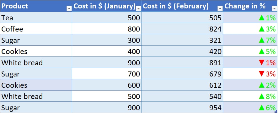
10. If you want to add colors, you can format data like this [green]▲0%, [red]▼0%. Then, click OK to apply the format.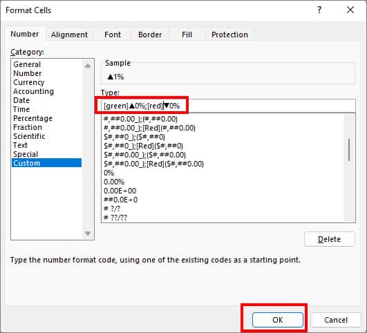 
    
11. Now, your data should look like this.
    

Using Conditional Formatting

If you want to insert arrows as per the custom rules, you can use Conditional Formatting.

1. Go to Excel and highlight cell ranges.
2. Click on the Home tab.
   
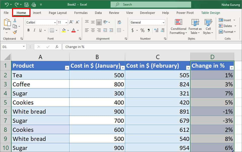
3. On the styles menu, choose Conditional Formatting > New Rule.
   
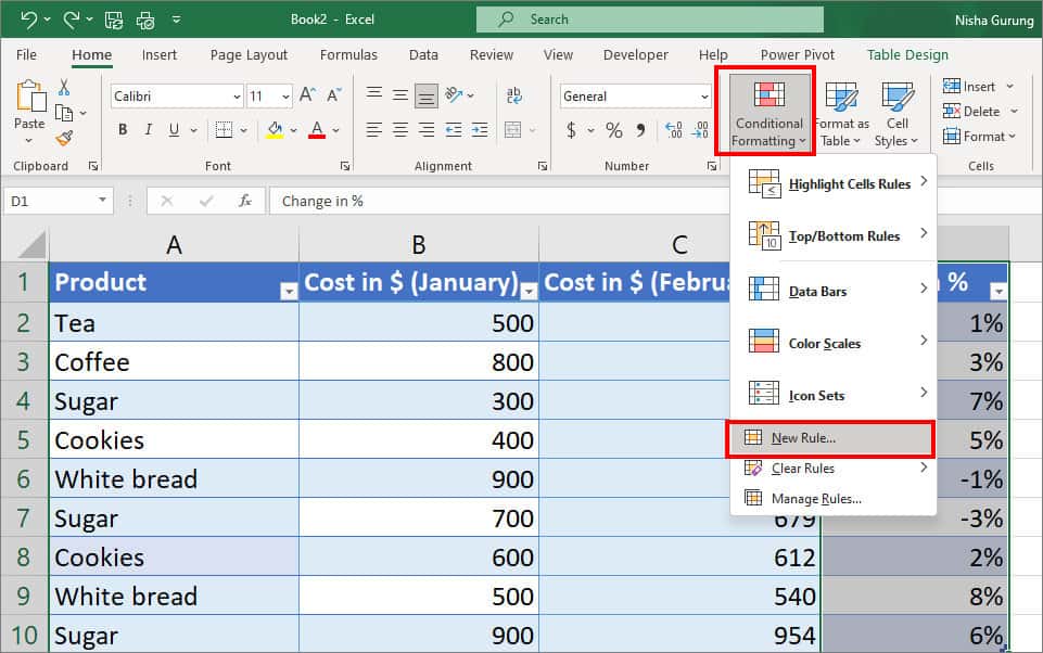
4. Pick Format all cells based on their values. 
   
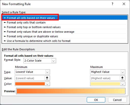
5. Now, on Format Style, choose Icon Sets from the drop-down menu. Then, on Icon Style, pick Arrows. 
   
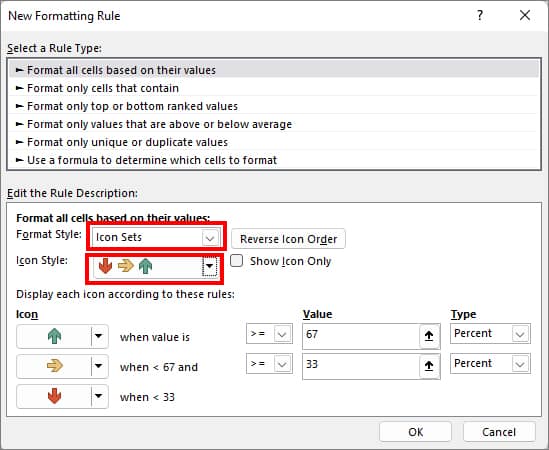
6. Check the box for Show Icon Only.
   
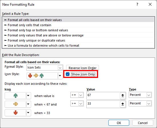
7. On the Icon menu, click on the Drop-down menu next to the yellow arrow. Choose No Cell Icon. (This is optional. Apply this only if you want to have red and green arrows)
   
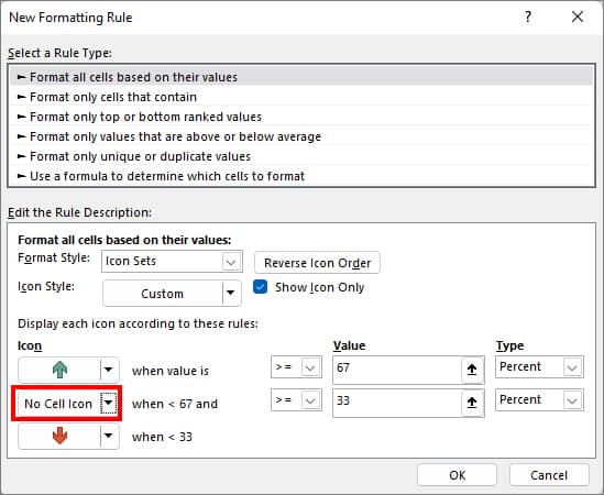
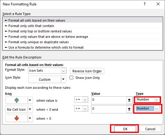
8. Under the Type menu, click on Number and choose OK.
   
9. Your data will have these trend arrows.
   

Insert Arrow in Excel Chart

For some Excel Charts, an arrow can help you provide a more obvious graphical presentation than the actual chart graph. 

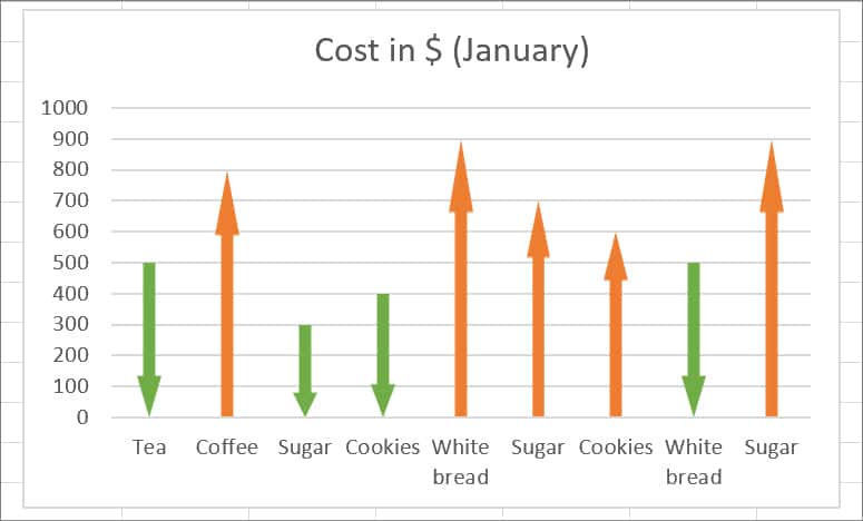
In the provided example, let’s suppose, you have a column chart and you want to illustrate the increasing or decreasing trend of data. You can take a look at the difference in the image itself. Picture A has a default Column Chart and Picture B has an Arrow. 

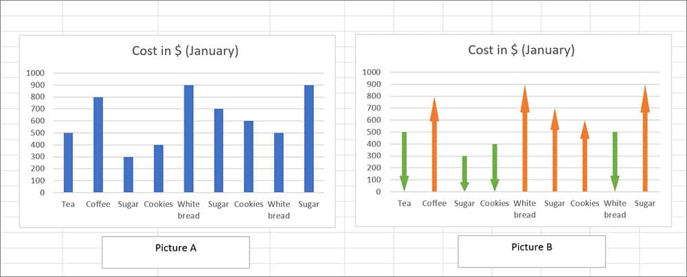
Now, to insert arrows to the chart, 

1. Firstly, navigate to Insert Tab.
2. On Illustrations, click on Shapes.
   
3. Under Block Arrows, pick Up Arrow. 
   
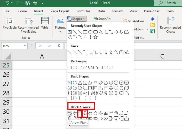
4. Now, draw the Shape in your worksheet and apply Colour as per your wish. Repeat the same step for Down Arrow.
    
5. Select any one Arrow. Then, enter Ctrl + C to copy.
   
6. Highlight Column Chart and enter Ctrl + V keys to paste the shape.
7. To insert a down arrow, click on a Single column and paste the arrow. Now, you can have arrows instead of bars in the column chart. 
   

Insert Arrow to Trace Formula

You can also insert an arrow to check and point out formulas. For this, you do not have to add any arrow shapes or symbols. Instead, we will simply navigate to the Trace Precedents or Trace Dependents menu.  

Precedent cells are the cells that your formula contains. For example, if you click on D2 which has a formula with =C2 and = B2 cells, C2 and B2 will be a precedent cell for D2.

To add arrows, highlight D2. Navigate to the Formula tab and click on Trace Precedents.

Dependent cells are the cells that the formula depends on. For example, if you click on cell B2, it will refer to the cell with the formula that has B2 cell. In our case, it will point to D2 as it is a dependent cell.

To insert arrows, select the B2 cell. Go to Formula Tab > Trace Dependents.

If you want to remove arrows, click on the Remove Arrows option under the Trace Dependents menu.