INDEX Function in Excel – How to Use it

If you’ve been using Excel for quite some time, you must’ve seen the INDEX and MATCH combination. The INDEX function is one of Excel’s many lookup functions and is popularly used with the MATCH function as an alternative to the VLOOKUP function.

The INDEX function is pretty simple to use by itself. All you have to do is specify the location of the data you want INDEX to return. In this article, we will be looking more into the arguments used in the INDEX function and look at examples.

Arguments Used in INDEX

The INDEX function requires two arguments and optionally takes two arguments. However, unlike most lookup functions like OFFSET, you cannot enter negative values. Your argument must be greater than zero, or else you’ll end up with the #VALUE! Error.

You can also enter multiple arrays using the INDEX function. However, before you pass the values for the function to retrieve a value, you must specify the array you wish the function to look for values.

Here is how you can enter the INDEX function in a formula:

=INDEX(array, row number, [column number],[area number])

• array: The range your value is located in.
• row number: The row your value is located in.
• [column number]: The column your value is located in.
• [area number]: If you’ve entered multiple areas, specify which area you wish to conduct the lookup.

Application of the INDEX Function

INDEX can be used in a number of ways. For starters, you can use the function as it is to retrieve a value from the specified range. You could also take it a step forward by nesting it with the MATCH function to conduct an even more complex lookup.

Example 1: Use INDEX to Return a Value From One Area

Let’s start by using INDEX to return a value from a single area. In this example, we will be passing only one range, therefore, there is no need to set the area number.

In this table, we have three rows and three columns (excluding the headers). Let’s use the INDEX function to return the total sales done by Jason on Monday.

=INDEX(B2:D4,3,2)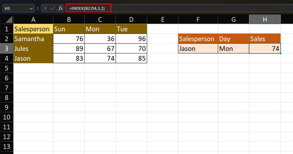

Example 2: Use INDEX to Pass Multiple Range

While you can pass multiple ranges using the INDEX function, it will only retrieve value from one area. The first area you specify in the array section will be numbered as the first area, and the rest will follow the same numeration. Depending on which area you wish INDEX to return values from, you must enter the appropriate value in the area number section.

In this spreadsheet, we have a single table. However, we wish to exclude row number 4 while conducting our lookup. Therefore, we will be setting two areas, B2:E3 and B5:E11 using INDEX to exclude row number 4.

Let’s retrieve data from Lynn’s Math scores from the data table. Here is how will be constructing the formula using the INDEX function to do so:

=INDEX((B2:E3,B5:E11),2,3,2)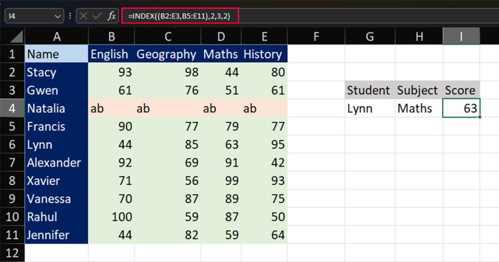

Example 3: Nest INDEX with MATCH

Now for one of the most popular function combinations in Excel. The INDEX function supports nesting other functions inside the function. You can use INDEX and MATCH functions to conduct complex lookups that even powerful lookup functions like VLOOKUP fail to perform.

Before we head on with this method, let me give you a brief overview of the MATCH function. MATCH is yet another lookup function in Excel used to return the position of a specified value in the range. MATCH is nested inside the row reference section of the INDEX section.

Here are the arguments used by the MATCH function in Excel:

=MATCH(lookup_value, lookup array, [match type])

• lookup_value: The value you wish to generate the location for.
• lookup_array:  The array with your data.
• [match type]: Specify if you wish to generate an exact match(0), lesser match(1), or greater match (-1).

In this spreadsheet, we have a table with ten rows and three columns. We will be nesting the INDEX and MATCH functions to create a lookup to look for the fruit that cost us $1.75. Here is the formula we will be using to navigate this:

=INDEX(A2:A10,MATCH(E4,B2:B10,0))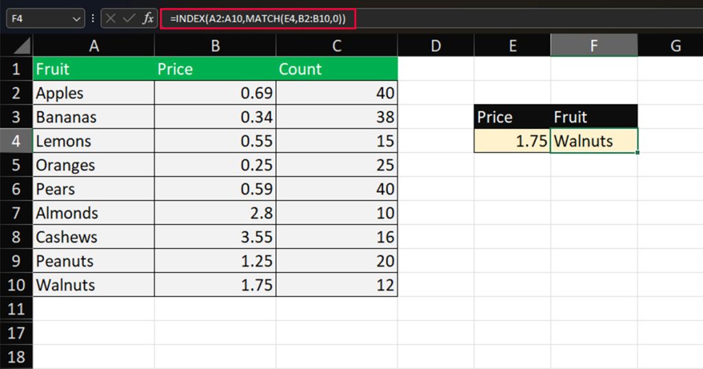

Let’s look more into this formula: