Excel’s IF function is extremely useful to test criteria and return the specified value when the value is True or False. I personally use this function on a day-to-day basis to return Yes/No, Completed/Pending, Good/Bad, and so on. But, its only drawback is you cannot test more than one criterion with the IF function.
You’re lucky if the IFs function is available in your Excel version to test the multiple conditions. However, even if it isn’t, you could always nest the IF function with IF. Or, use IF with other logical functions such as AND and OR nested together.
Arguments for the IF function
Excel’s IF function takes up the condition and values to return as function arguments.
Syntax: IF(logical_test, value_if_true, [value_if_false])- logical_test: condition you want to test with TRUE or FALSE logic
- value_if_true: the value you want to return when the logical test is TRUE
- [Value_if_false]: the value you want to return when the logical test is FALSE
Note that the arguments placed inside the [] brackets are optional.
How to Use the IF Function With 3 Conditions
Method 1: Nest IF inside IF
Firstly, you can actually nest the IF function inside IF. By nesting IF statements, you could create as many conditions to test as you want. To check 3 conditions, we will nest IF two times inside the IF function.
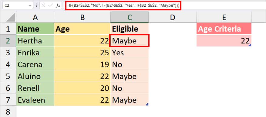
Example: Suppose you have an Excel record of Name and Age. You need to check if they’re eligible, not eligible, or could be eligible. For this, you have three different conditions to test and return the value:
- Return “No” if the value is less than the age criteria
- Return “Yes” if the value is greater than the age criteria
- Return “Maybe” if the value is equal to the age criteria
To find out, use the formula given below.
=IF(B2<$E$2, "No", IF(B2>$E$2, "Yes", IF(B2=$E$2, "Maybe")))
As you can see in the formula, we have passed down three different criteria in the IF function. In our logical test, we’ve locked cell $E$2 to make it an absolute cell. This way the other cells will look only at the value of the E2 cell for logical comparison.
Since the value of cell B2 exactly matches with the E2 cell, it returned Maybe. While the cell is still selected, extend the flash-fill handle to return the values in other cells.
Method 2: Nest AND Function inside IF function
Similar to the IF function, AND function is also a logical function used to test the conditions. You could nest AND function inside the IF function to test three different conditions. Use this formula when all three conditions need to be either True or False.
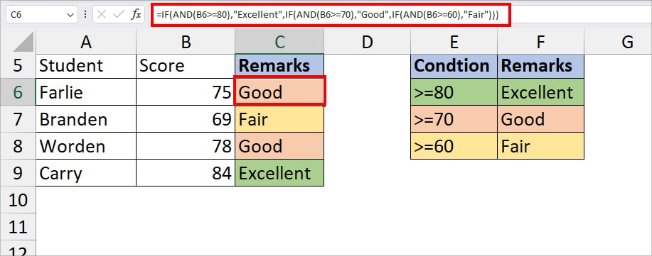
Syntax: IF(AND(logical1, [logical2] [logical3]), value_if_true, [value_if_false]))Example: Let’s assume you have the History test scores of Grade 2 students in your worksheet. You need to provide remarks to the students based on their test scores. According to the school’s standard remark rule, the conditions are:
- Excellent: Scores greater than or equal to 80
- Good: Scores greater than or equal to 70
- Fair: Scores greater than or equal to 60
Now, you can use this formula to evaluate the remarks of students
=IF(AND(B6>=80),"Excellent",IF(AND(B6>=70),"Good",IF(AND(B6>=60),"Fair")))
In the formula, IF(AND(B6>=80), “Excellent” is your first condition. IF(AND(B6>=70), “Good” is the second condition, and IF(AND(B6>=60),”Fair”) is third condition.
The AND function returns either TRUE or FALSE for each condition. Then, the IF function returns “Excellent” if the value is TRUE. Similarly, in case the value is FALSE, it returns either “Good” or “Fair.” In our case, it returned Good. Use the Flash-fill to return values in the remaining cells.
Method 3: Nest OR function inside IF function
OR function is another logical function that returns TRUE or FALSE values whenever you test a certain condition. With IF and OR functions nested together, you could test three criteria for your data. This function is useful when one of the three conditions can be either True or False.
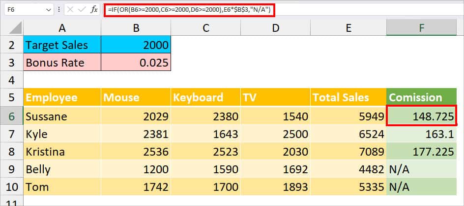
Syntax: IF(OR(Something is True, Something else is True), Value if True, Value if False)Example: You have a list of employees and their total sales of each item. Based on their sales performance, each employee will get a 2.5% commission from their total sales. There are three conditions you need to test to decide whether the employees should get a commission or not.
- Sales of Mouse must be greater than or equal to 2000.
- Sales of Keyboard must be greater than or equal to 2000.
- Sales of TV must be greater than or equal to 2000.
To test, enter the IF and OR formula in the box.
=IF(OR(B6>=2000,C6>=2000,D6>=2000),E6*$B$3,"N/A")
In the given formula, the OR function will first check whether the values of B6, C6, and D6 are greater than or equal to the Target. Then, it returns TRUE or FALSE based on all three conditions.
Now, the IF function will return the Total sales *2.5 % commission if the value is True. Or, “N/A” if the value is False. Since it was true, the formula returned 148.725 commission in the cell.
Drag down the flash-fill to return results in other cells too.
Alternative to using IF function with multiple criteria
If you have access to the IFs function, you do not have to go through the hassle of nesting several logical functions with IF. Excel’s IFs function is a new function that checks multiple criteria. It is available in Excel 2019 and later versions.
Syntax: IFs(logical_test1, value_if_true1, [logical_test2, value_if_true2], [logical_test3, value_if_true3])The functionality of the IF function is pretty much similar to the IF function. You can pass down the criteria and value to return to when true or false. The only difference is you can enter multiple criteria which is up to 127 in maximum.