If you need to find out the rank of a certain number in Excel, you’d have to sort them in order first. But, with Excel’s RANK function, you can quickly return the position of the number without rearranging them. One of its best functionality is that you can check the rank of a value in both ascending and descending order.
Arguments for RANK Function
Excel’s RANK function returns the position of the number from the array of ranges. You can find out the rank of a number in ascending or descending order.
Syntax: RANK(number,ref,[order])The RANK function takes only three arguments.
- Number: Cell reference or the number to find out its position. [Required]
- Ref: List of numbers to rank the number from. [Required]
- Order: Rank number in ascending or descending order. [Optional]
- 0: Descending order (Highest to Lowest)
- 1: Ascending order (Lowest to Highest)
For Example, we have 8, 5, 7, 3, 4, 2, 9 numbers in the data from cell B2:B8. To find out the rank of the number 7 we entered the formula as
=RANK(7, B2:B8, 1)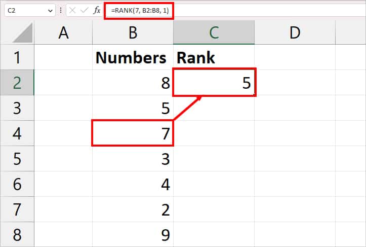
Since we passed down 1 argument in the formula, it sorts the number in ascending order (lowest to highest) first. Then, compares the position of 7 with other numbers and returns the 5th rank as an output.
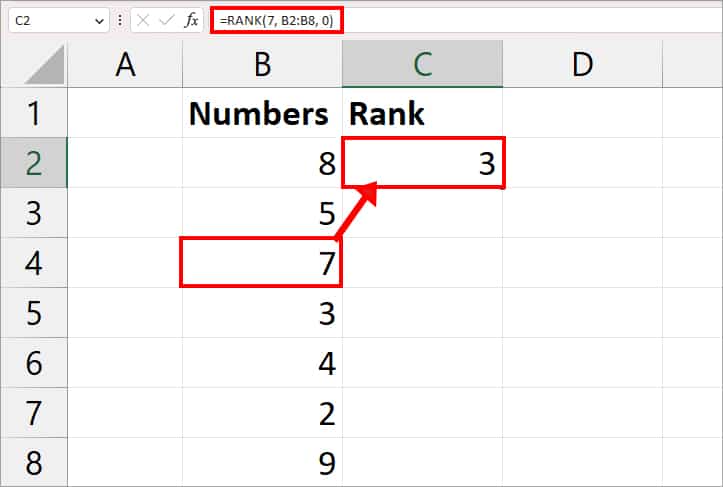
Similarly, if we wanted to find out the position in descending order, the formula would be =RANK(7, B2:B8, 0) . Now, the rank of number 7 will be 3.
What Should You Know Before Using the RANK Function?
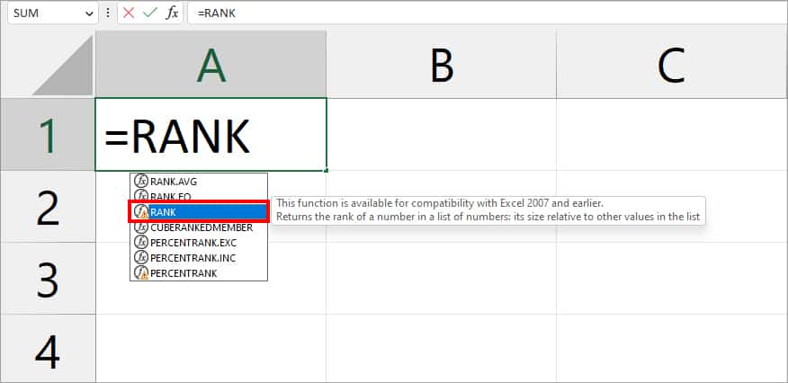
The RANK function falls under the compatibility functions. Meaning, Excel has introduced its newer versions such as RANK.AVG and RANK.EQ functions with improved functionality. So, Excel might completely remove the RANK function in the upcoming versions.
At the time of writing this article, the RANK function still supports Excel 2016 and later versions. However, when you attempt to use it, you can see a yellow exclamation error in the function name.
How to Use RANK Function in Excel?
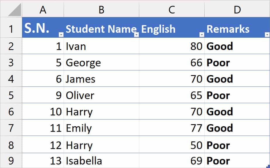
Let’s suppose, I have the English test scores of students in a spreadsheet. We will find out the rank of these scores in different cases.
Case 1: Rank Number in Ascending Order
Here, we will check the rank of a student named Emily. We have highlighted the row for a more clear picture. Now, to find out the rank, we used the formula as
=RANK(C7, C2:C9, 1)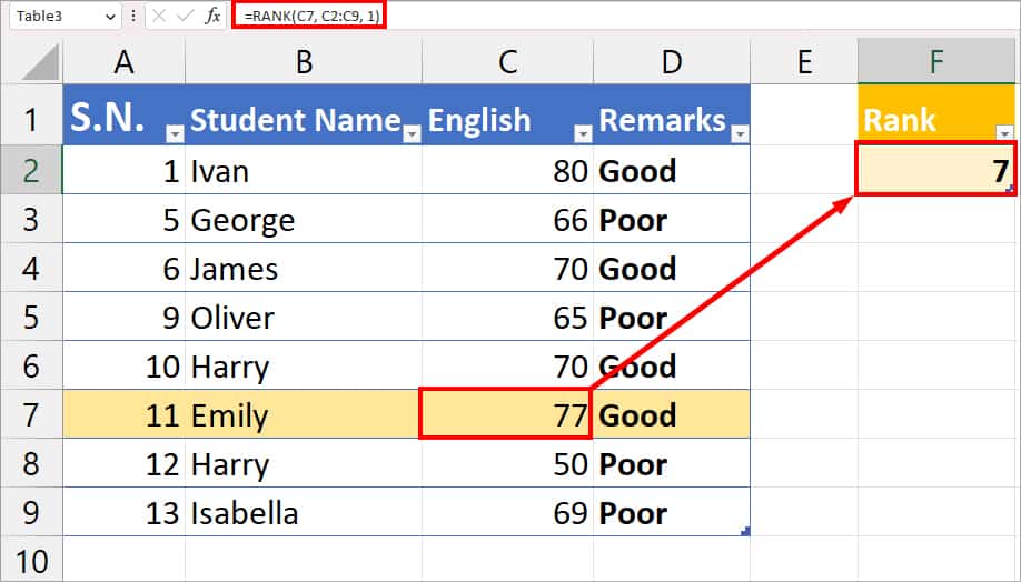
The formula compared the value of C7 (77) with other number ranges from C2:C9 in ascending order. Then, it returned 7th rank.
Here, we’ve taken the cell reference as a number in the formula. Note that if you want to use the flash-fill for other cells, you should lock the cells with references. For Instance, C2:C9 is a reference cell, you’d have to enter it as $C$2:$C$9 to make it an Absolute Cell.
Case 2: Rank Number in Descending Order
Again, let’s rank the same test score but in descending order. For this, we will enter a different order in the formula which is
=RANK(C7, C2:C9, 0)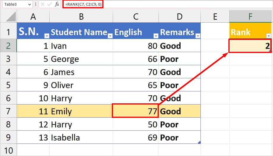
This time the formula will return the 2nd position in descending order.
Case 3: Rank Without Specifying the Order
The Order argument is optional in the RANK function. But, what value would you get if you did not specify the order? To check this, let’s find out the position of cell C3 with the given formula.
=RANK(C3, C2:C9)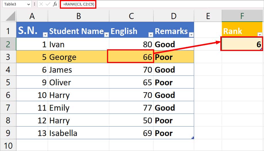
In the formula, we haven’t specified the order to rank. So, Excel will take 0 by default and return the rank in descending order which is highest to lowest value. We got 6th rank as a result.
Case 4: Rank Duplicate Value
There can be instances when you have duplicate values in the numbers. During such situations, you will get the same rank for both numbers.
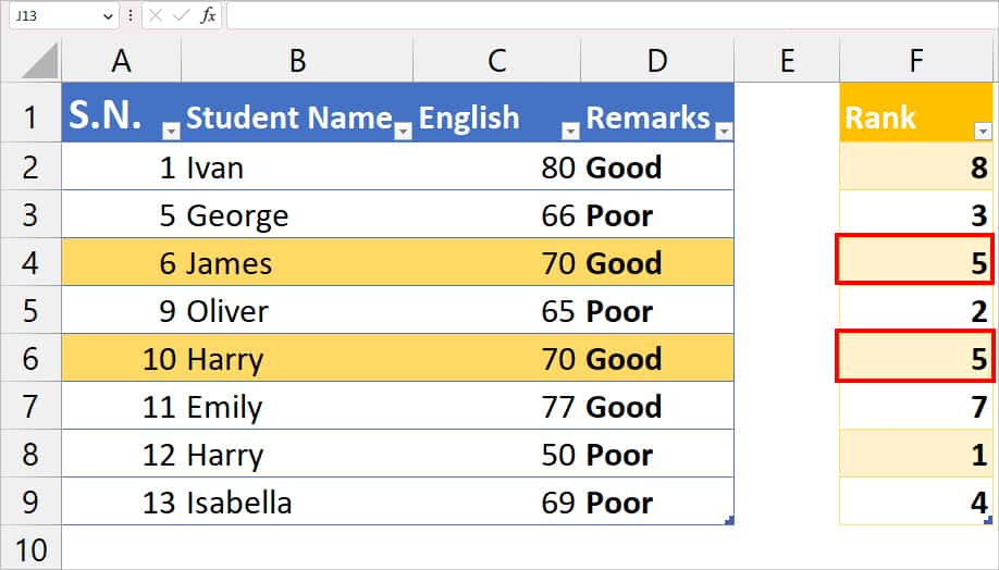
In our case, cell C4 and cell C6 have a duplicate value of 70. So, if we used the given two formulas, we’d get the same position which is 5th in ascending order.
=RANK(C4, C2:C9, 1)
=RANK(C6, C2:C9, 1)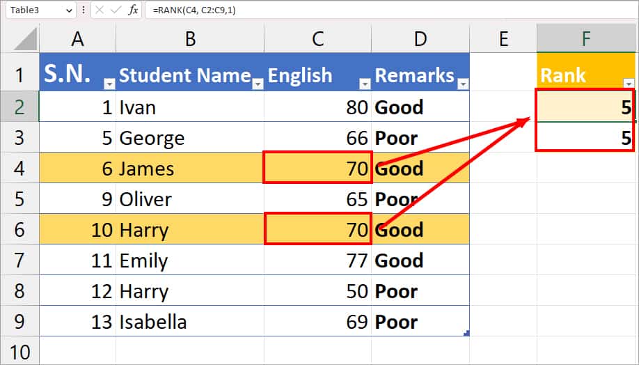
You must note that when you have duplicate values, you won’t have the sequential rank. For Example, we got a rank of 5 as a tie above. Now, for the next number which is in ascending order, we will get the 7th rank. You can see in the given picture, Excel skipped the 6th position.
How to Avoid Errors While Using the Rank Function in Excel?
In most cases, users often encounter #VALUE! Error and #N/A error while using the RANK function. The RANK function takes only the number values in the arguments. So, when you reference a non-numeric value in the formula, it’ll return these errors. To avoid this, check and make sure to enter the number in the cell.