How to Unpivot Data on Excel

While pivoting data makes it look concise, you may not always find the range easier to analyze. In case of a larger data range, manually unpivoting data can take you quite a while. Fortunately, Excel can automate this task for you using the Power Query.

The Power Query is a powerful tool in Excel used specifically to automate tasks. The Power Query is available from the Excel version 2016 and later. You can unpivot columns in the Power Query interface, then load the data to your Excel sheet.

We have divided the methods into three easy steps, so follow along with this guide and unpivot your data in no time!

Step 1: Convert Range to Table

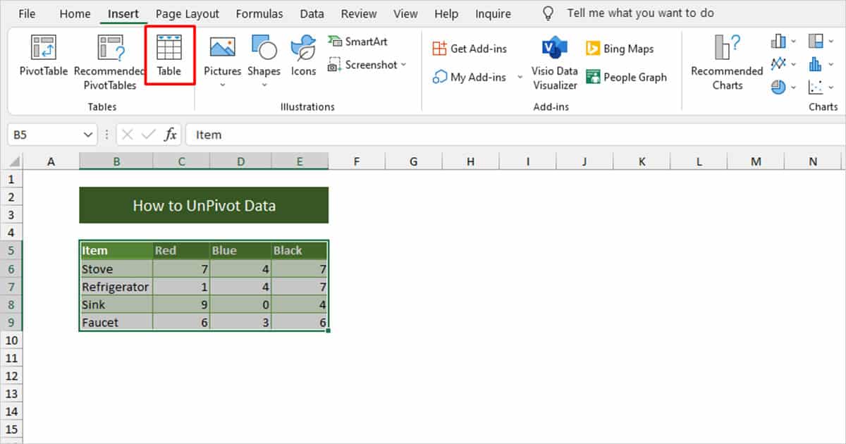
You will first have to transform your range into a table before you can load it to Power Query. Select your range, then use the Excel shortcut Ctrl + T to convert it to a table. You can also navigate through the ribbon to change the range to a table:

1. Select the range.
2. Head to Insert.
3. From the Tables section, click Table.
   

Step 2: Load Data in Power Query

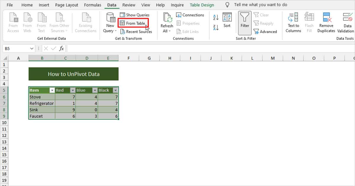
After you have converted your range to a data table, you can load the table to Power Query.

1. Select any cell from the table.
2. From the menu bar, click on Data.
3. Select From Table in the Get and Transform section.
   

Step 3: Unpivot Columns from Power Query

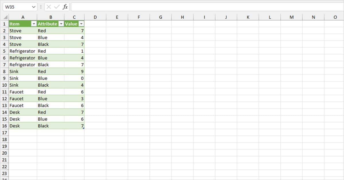
When your data loads in the Power Query editor, you can go ahead and unpivot your values. 

1. Select the column you wish to unpivot. If you wish to unpivot multiple columns, hold down on the SHIFT key and click on each column.
2. Right-click on the column header and select Unpivot Columns.
   
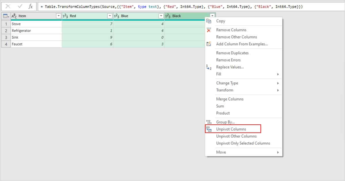
3. Optional: Change the column header by double-clicking on it. 

Step 4: Load Data Back to Worksheet

You will need to close and load the data in the Excel window, once you unpivot your data.

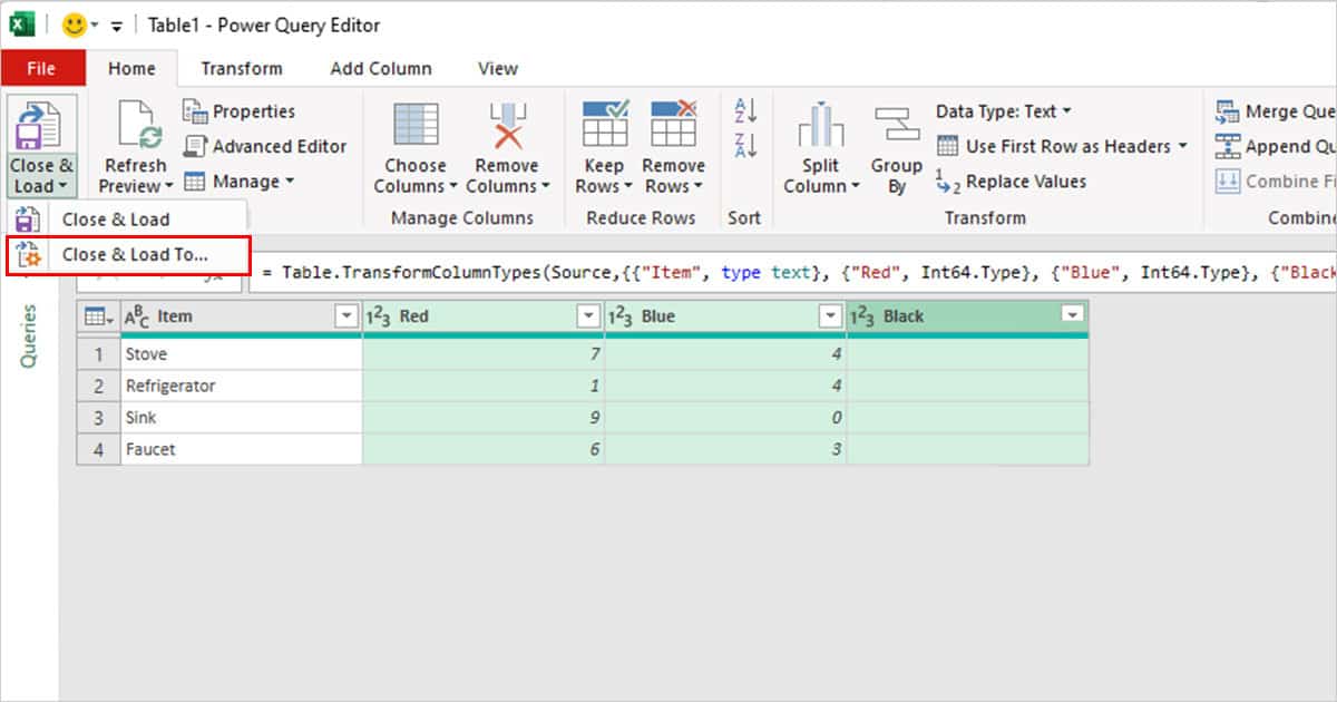
1. Head to the Home tab.
2. Select the fly-out under Close and Load > Load to.
   
3. From the Load To window, select the box next to Table.
4. If you want Excel to create a new worksheet for your data, select New worksheet. Else, specify the range after choosing Existing worksheet.
   
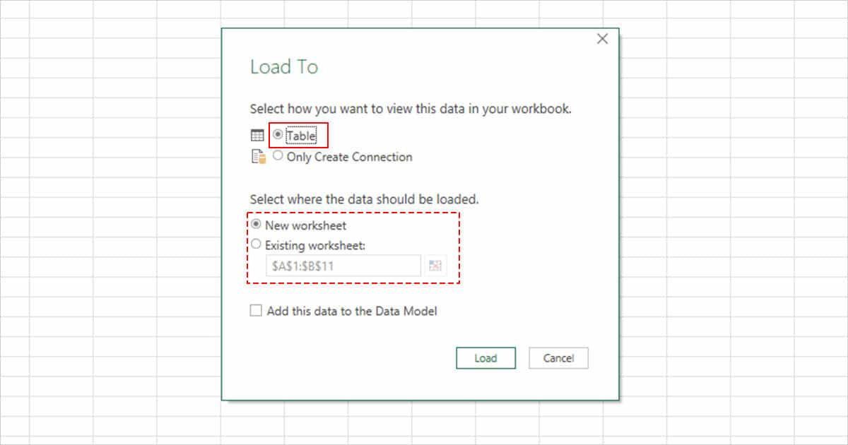
5. Click Load.
   

Other Unpivoting Options

In Power Query, you could’ve noticed two other options excluding the Unpivot Columns option. These options are no different, they only differ in terms of selection. Here’s a little breakdown of each of the two options if you’re curious:

• Unpivot Other Columns: This will prompt the Power Query to unpivot the unselected columns. For example, if you’ve selected the first column, every column except the first one will get unpivoted.
• Unpivot Only Selected Columns: When you select this option, Excel will unpivot only the selected columns.

Conclusion

Although using Power Query might sound a bit intimidating when you’re just starting our Excel, it is actually pretty simple. The simple interface of the Power Query makes it extremely easy to navigate.

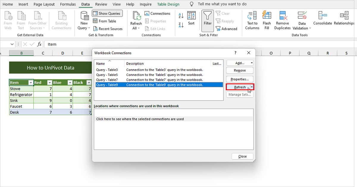
What I love most about using Power Query is that it is dynamic. For any data you add more to the data table, Excel automatically pivots it once you refresh your data.

1. After making changes in the table, head to the Data tab.
2. Select Connections from the Connection section.
3. Choose your table from the Workbook Connections window.
4. On your right, click on Refresh.