How to Sum an Entire Column in Excel

Excel allows you to instantly sum an entire column in Excel using the AutoSum command. Also, if you want to manually sum a column, you can use the SUM function in Excel.

If you have your data in an Excel table, use the Table Row feature to sum columns. For columns that are filtered, use SUBTOTAL instead of SUM to sum only visible data.

Use AutoSum to Sum a Column in Excel Instantly

The AutoSum feature automatically detects numbers in a column and calculates its total. You can find and insert AutoSum from Excel’s Home tab or use a shortcut.

For AutoSum to work, select the cell directly under your column. Then, head to Home > AutoSum or enter the following shortcut:

Alt + =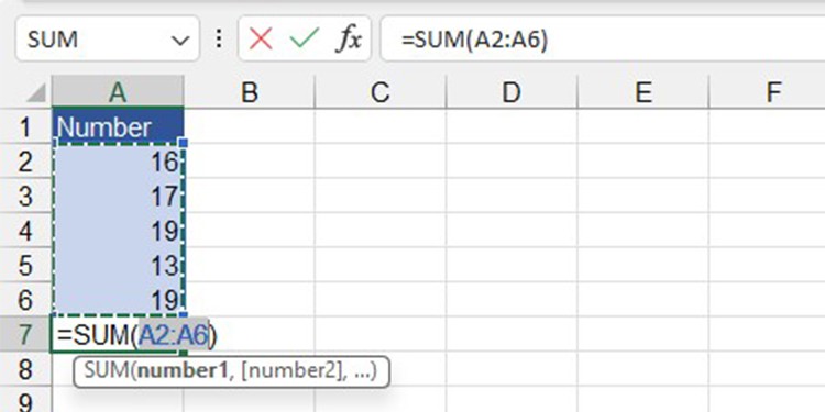

Check if all cells from your column are selected in the formula, then hit enter.

Use the SUM Function to Sum a Column in Excel

You can also directly enter the SUM function instead of using AutoSum to calculate a column’s total.

The SUM function is pretty easy to use and takes arrays as arguments, meaning you simply have to enter the range to calculate the total.

Here is the syntax SUM function used in a formula:

=SUM(number1,[number2],...)

Take a look at this spreadsheet.

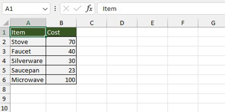
Column B holds the initial cost taken to manufacture an appliance. In column D, we need to calculate the total manufacturing cost of all five appliances.

In cell E2, I entered the following formula to calculate the total cost of manufacturing the appliances.

=SUM(B2:B6)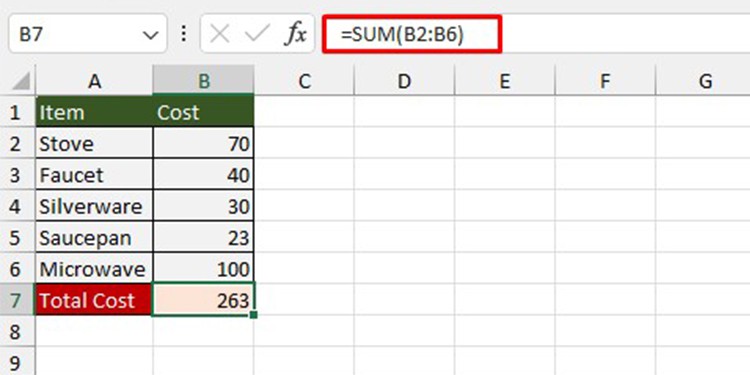

Sum a Column in Excel Table

If you have your data in an Excel table, add all cells in each column of the table.

Before you proceed, make sure your data is in a table. If not, select your range and press Ctrl + T. If you’ve included table headers, select My table has headers in the Create Table window, then click OK.

1. Select your table.
2. From the menubar, go to Table Design.
3. In the Table Styles Option section, check the box next to Total Row.
   
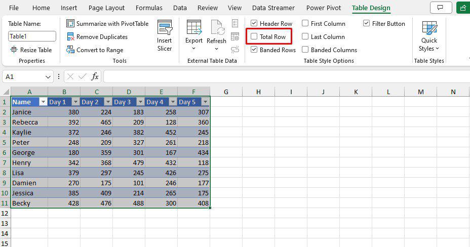
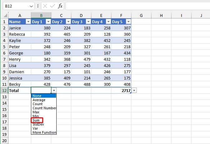
4. To calculate the sum of multiple tables, select the cell under each column. Once the fly-out appears, click on it and select Sum.
   

Sum Through Filtered Data Using SUBTOTAL

Oftentimes, we filter cells to focus on different values in Excel. Although the cells within the row remain out of sight, Excel takes them into account when generating the total.

If you wish to exclude the filtered in a column when adding, use the SUBTOTAL function instead of SUM.

Here’s what SUBTOTAL looks like when constructing a formula:

=SUBTOTAL(function_num, ref1, [ref2],...)

Take a look at this sheet.

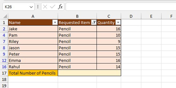
The original list contained 15 items. After filtering the table to only show the users who have requested pencils, the column only has 7 items.

Column C holds the number of pencils each person requested. Let’s use SUBTOTAL to count the total number of pencils requested.

On an empty cell, enter the following formula:

=SUBTOTAL(9,C2:C16)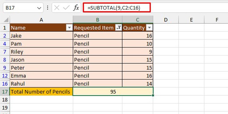

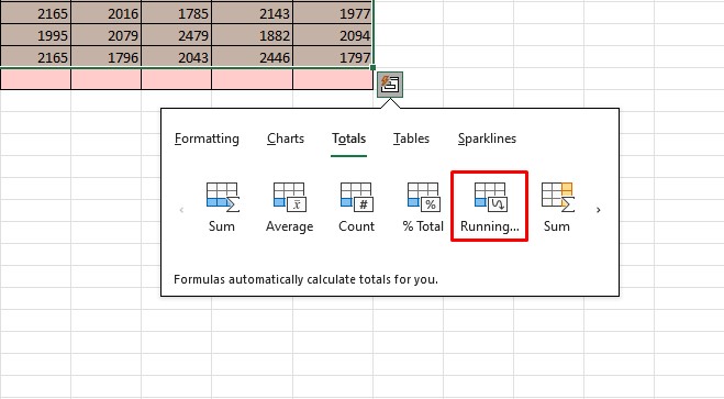
Use Quick Analysis to Generate Running Total

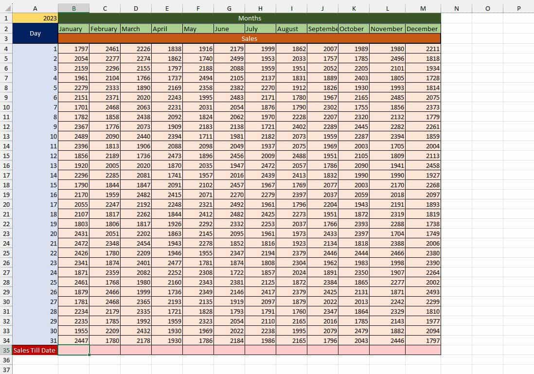
Say, you’re working on an annual sales sheet. You need to know how much running revenue your company has generated from each month up to December.

Using SUM to make this addition will be pretty time-consuming. Instead, use Excel’s Quick Analysis toolbar to generate a running total for all columns.

Here’s how I calculated the running total for the 12 columns in a sales sheet:

1. Select range B4:M34.
   
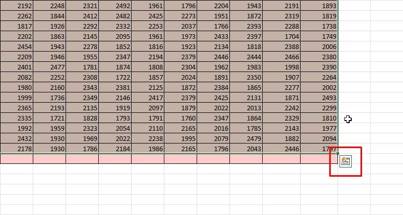
2. An icon will appear on the bottom-right corner, click on it. If it doesn’t, select Ctrl + Q.
   
3. Switch to the Totals tab.
4. Select Running.