When you’re dealing with decimal values, like percentile values, you might often find yourself in need of rounding them up. There are several reasons to round decimal values, of which, bringing the decimal to the closest whole number and decreasing the length of the decimals are more relatable.
Excel has four different functions to help you round up your numeric values. Each function has its own purpose when it comes to rounding up the figures. In this article, we will go into detail about each function, and how different arguments result in different values in Excel, so keep reading!
Use the ROUND Function
When you use the ROUND function, Excel follows the standard rule of round-offs. This means, if you wish to round your value off by one decimal, Excel will increase the value of your digit by one only if the digit on the right is 5 or more than 5. For instance, 7.85 will return 7.9, and 8.91 will still return 8.9.
Arguments Used in ROUND
Let’s get into the arguments used by the ROUND function:
=ROUND(number, num_digits)- number: The digit you wish to round off
- num_digits: How many digits you wish to round your number by
You can enter both negative and positive numbers in the num_digit section. If you insert a negative number, for instance, -1, it will round your value to the closest value divisible by 10 (in the case of -1). Serially, -2 will round it off to the closest 100th value and -3 will round it off to the closest 1000th value.
Entering 0 in the num_digits section will convert your value to the closest whole number while, if you enter a positive number, it will keep the equal number of digits after the decimal point. Whether or not to increase the last digit is completely based on the rule of round-off.
Examples
The best way I can elaborate on these arguments is through examples. Take a look at this table below to see what argument results in what value in the ROUND function.
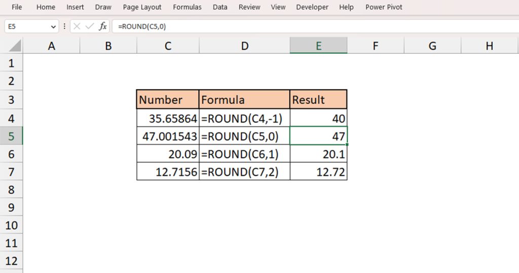
| Number | Formula | Result |
| 35.65864 | =ROUND(C4,-1) | 40 |
| 47.001543 | =ROUND(C5,0) | 47 |
| 20.09 | =ROUND(C6,1) | 20.1 |
| 12.7156 | =ROUND(C7,2) | 12.72 |
We rounded off the first value by -1 in row 1. This brought the number 35.65864 to the closest tenth value, 40. Similarly, as we used 0 in the num_digit section in the second row, it rounded our value to a whole number.
In the third row, the number 20.09 was rounded off by one digit. The first digit after decimal is 0 while the second is 9. As 9 is greater than 5, this will increase the value of 0 by one digit to 1. Therefore, this resulted in our value: 20.1. This is the same as the value in the fourth row.
Use ROUNDUP Function
In contrast to the ROUND function, ROUNDUP does not follow the round-off rule. Instead, this function will up the rounded-off value by one digit.
Arguments Used in ROUNDUP
The ROUNDUP function has the same arguments as the ROUND function. Here is the format you can use to enter the ROUNDUP function into a formula:
=ROUNDUP(number, num_digit)- number: The digit you wish to round off
- num_digit: The position of the decimal you wish to round up the value
Entering a negative or positive value in place of the num_digit section will work just as the ROUND function. However, it will only increase your rounded value.
Examples
Here are some examples of how the ROUNDUP shows different results according to the argument passed.
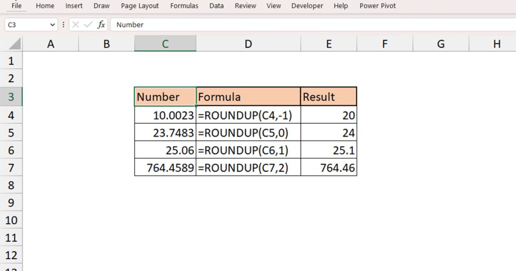
| Number | Formula | Result |
| 10.0023 | =ROUNDUP(C4,-1) | 20 |
| 23.7483 | =ROUNDUP(C5,0) | 24 |
| 25.06 | =ROUNDUP(C6,1) | 25.1 |
| 764.4589 | =ROUNDUP(C7,2) | 764.46 |
Use ROUNDDOWN Function
The ROUNDDOWN function is the exact opposite of the ROUNDUP function in Excel. Instead of increasing the set digit, the ROUNDDOWN function will decrease the digit by a digit. However, there is one similarity both ROUNDDOWN and ROUNDUP function share, and that is they both don’t follow the round-off rule.
Arguments Used in ROUNDDOWN
You will have to enter two arguments, including the number and the round-off value in the ROUNDDOWN function. Here’s the syntax:
=ROUNDDOWN(number, num_digit)- number: the number you wish to round off
- num_digit: the position of the value you wish to round down
You can enter positive, negative, or zero digits in the num_digit section. A positive value will reduce the digit from the position equal to the set number, entering a negative value will round down your number to the nearest tenth value, and zero will change the digit to a whole number.
Examples
Here is how different arguments will produce different values using the ROUNDDOWN function.
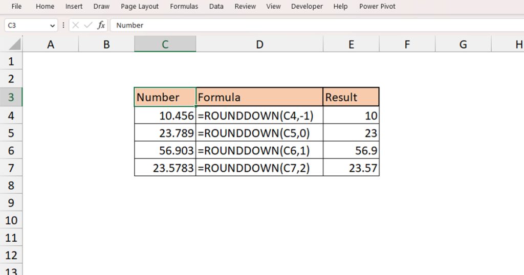
| Number | Formula | Result |
| 10.456 | =ROUNDDOWN(C4,-1) | 10 |
| 23.789 | =ROUNDDOWN(C5,0) | 23 |
| 56.903 | =ROUNDDOWN(C6,1) | 56.9 |
| 23.5783 | =ROUNDDOWN(C7,2) | 23.57 |
Use MROUND Function
The MROUND function is a bit different than the rest of the round functions. You can use this function to round your value to the nearest multiple of the set value. You can use MROUND when you wish to generate a value that is divisible by the same number.
Arguments Used in MROUND
MROUND takes in the same number of arguments as the other round function. Here is what the function looks like when written in a formula:
=MROUND(number, multiple)- number: the value you wish to round off
- multiple: the number you wish to generate the multiple of
Contrary to other ROUND functions, you cannot enter negative values as multiples in the MROUND function. If you do, the MROUND function will return the #N/A error. You can enter any positive multiple, including zeros. However, entering zero will return you only zero.
Examples
Take a look at a few of the examples we’ve created using different arguments in the MROUND function.
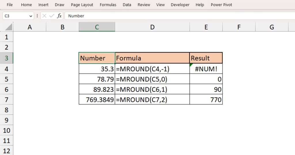
| Number | Formula | Result |
| 35.3 | =MROUND(C4,-1) | #NUM! |
| 78.79 | =MROUND(C5,0) | 0 |
| 89.823 | =MROUND(C6,1) | 90 |
| 769.3849 | =MROUND(C7,2) | 770 |