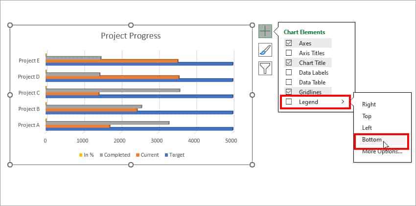
In Excel charts, Series represents the data value in a column or row that you used to plot charts. So, just by viewing the Series title, you can easily comprehend the data illustration of the graph like in the picture.
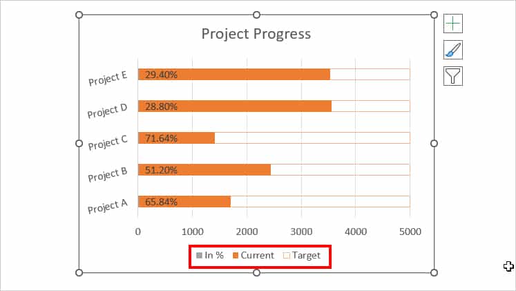
If you’ve selected the Column headings while plotting charts, these series appear in the same name as your column heading. But, if you’ve only selected the data range, Excel will name it “Series 1”, “Series 2”, etc, instead. Either way, if you are looking for a way to retitle the Series, you can follow these three easy methods.
From the Column Heading
If you’ve created the charts along with the Column header of the data, we have the quickest method to rename the series. Since you will have the same Series title in your charts, you could change the name in the Sheet itself. When you do this, Excel will automatically update the series name in the chart too.
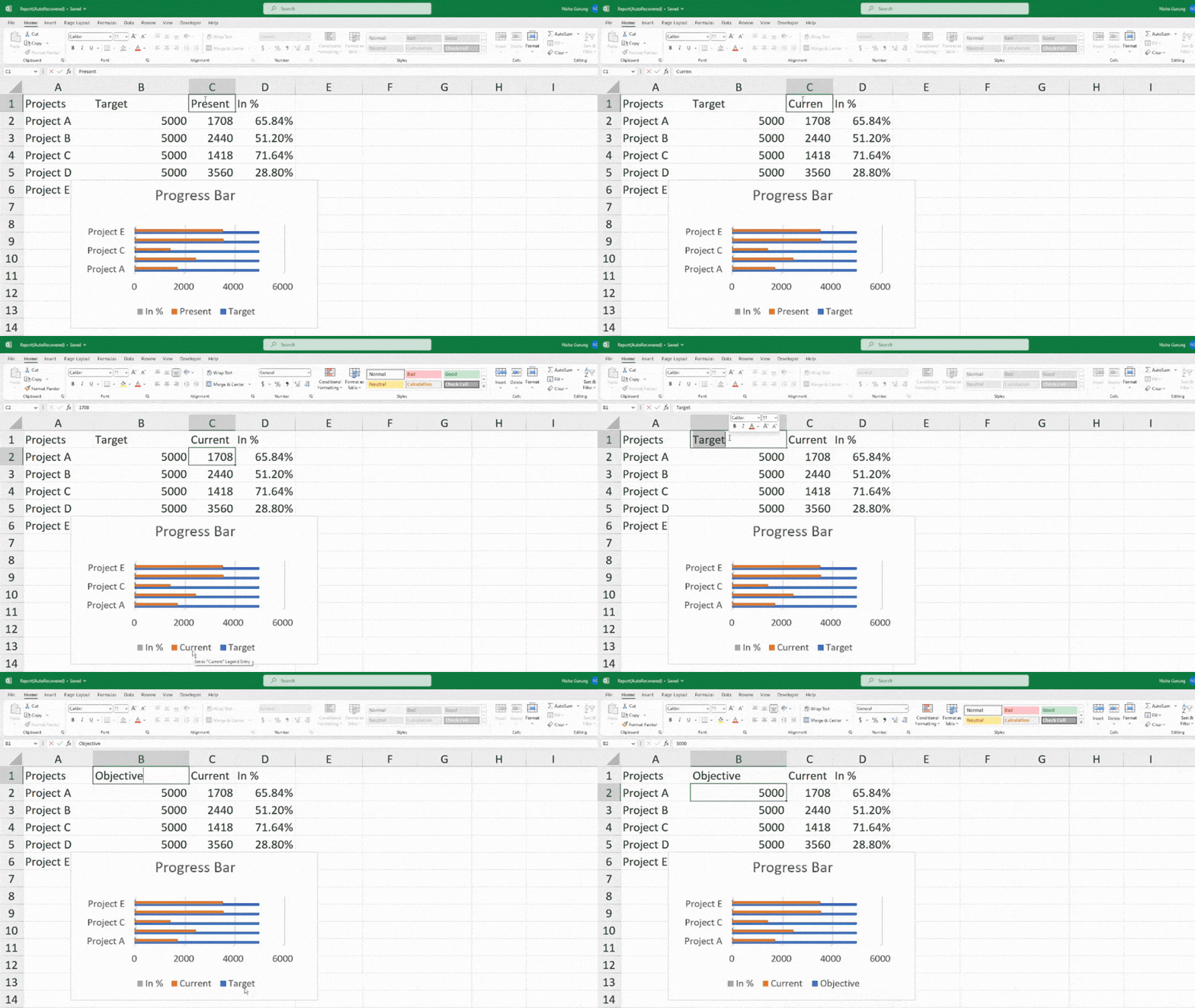
However, note that this method does not work if you’ve plotted the charts with data range only.
From Chart Filters
For users who has Series1, Series2, etc as a Series name, you could use the Chart Filters icon to rename the series. It is the easiest way to retitle the series as you can instantly access the Filter icon in the Chart area itself. This approach is best for users who wishes to change the name of only one series at a time.
- Click on the Chart Area.
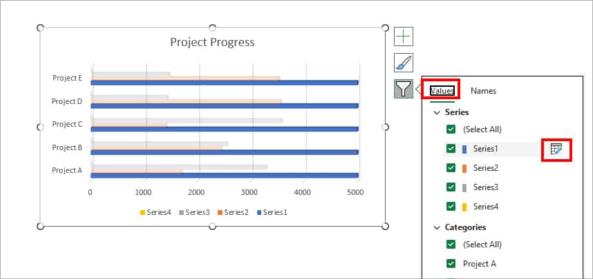
- Then, on the top-right corner of the Chart, click Chart Filters icon.
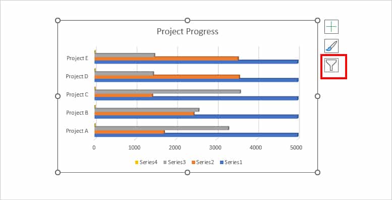
- Stay on the Values tab. Then, under the Series, hover over the series and select the Edit Series icon.
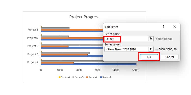
- On the Series name box, enter a New name and hit OK.
From Select Data Menu
If you’d rather wish to rename all series, I suggest you use the Select Data Menu. With the above method, you would have to keep going to the Filter icon for each series. But, here, you can change all of the names one by one and save them at once.
- Click on the Chart.
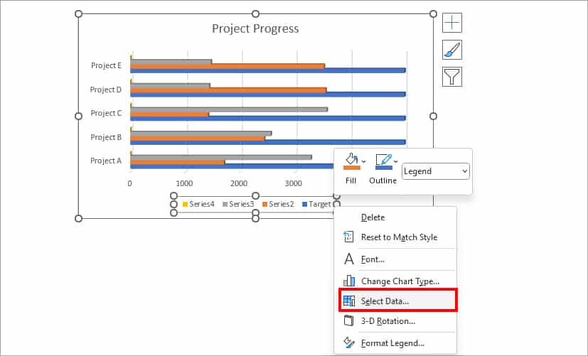
- Right-click on the Series and choose Select Data.
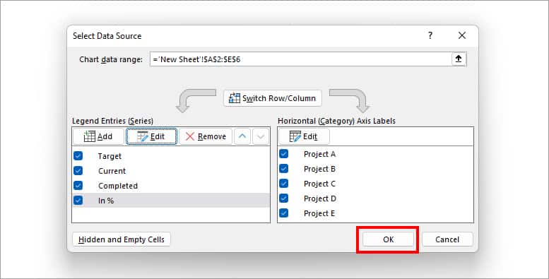
- Under Legend Entries(Series), select a series to change. Then, hit Edit.
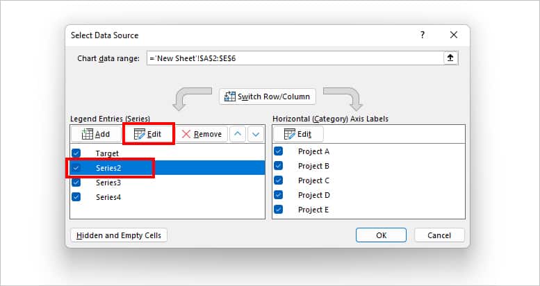
- On Series name, type in New name for the Series and click OK.
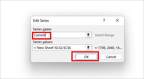
- Repeat steps 3 and 4 for the other series. When done, hit OK.
How to Format Series Title in Excel?
After renaming the series title, you can format them with different styles to have a more appealing look. You could change the font text, style, color, size, etc.
- Select the chart.
- Right-click on the Series Title and pick Font.
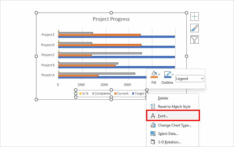
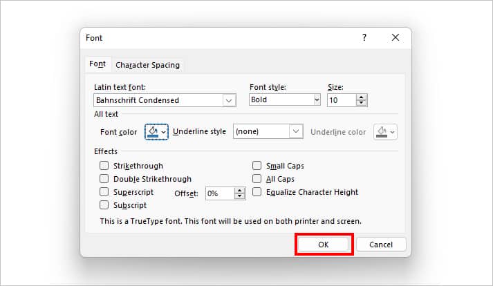
- On the Font box, choose your Font Text, Style, Size, Color, and Effects. Once you’re done, click OK.
How to Re-add a Series Title in Excel?
When you create an Excel chart, the Series will appear in the chart area by default. However, if you have deleted them, you could follow these steps to re-add the series title.
- Click on the Chart area and select the Chart Elements (+) icon.
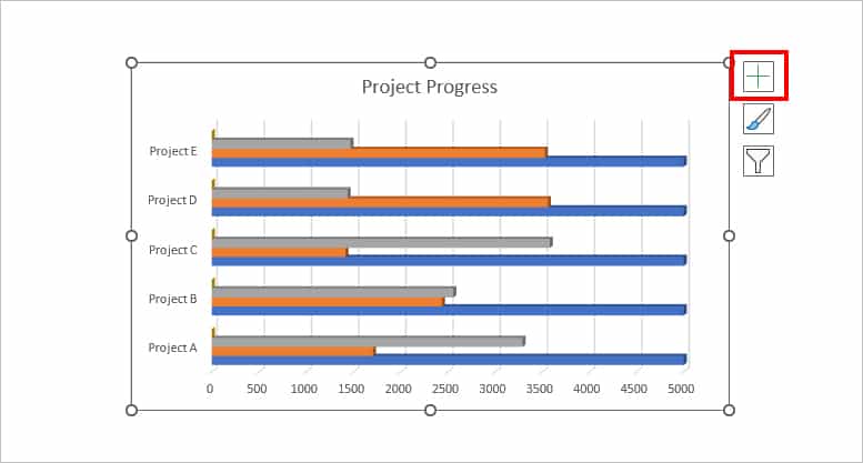
- Hover over the Legend option. Then, pick a Series position .i.e Right, Top, Left, Bottom.
