I think we all have been in situations where we’ve entered an extra character before or after our value. This especially happens when copy-pasting values directly to the Excel spreadsheet. There’s always one sneaky character, mostly space, that invites itself onto our data.
In bigger spreadsheets, it’s almost unimaginable to manually remove these redundant characters. I would normally use the Find and Replace command to remove such characters, however, this would get rid of all of these characters in the grid.
To remove the first or last characters in Excel, we will have to design formulas using the REPLACE, LEN, and MID functions. You could also opt for LEFT or RIGHT functions instead of MID while constructing your formula. We will be putting all of these functions into a formula to remove the first or last character in Excel, so keep reading!
REPLACE Function
The REPLACE function in Excel works by replacing a string with a new string value. This is done by specifying the position of the string in your text that you wish to replace. The REPLACE function is entered in the following format while writing a formula:
=REPLACE(old_text, start_num, num_chars_new_text)- old_text: The original text with the character you wish to replace.
- start_num: The position in the text you wish to replace characters from.
- num_chars: How many characters do you wish to replace in the data?
- new_text: The replacement character.
Use REPLACE to Remove the First Character
Let’s apply the following spreadsheet.
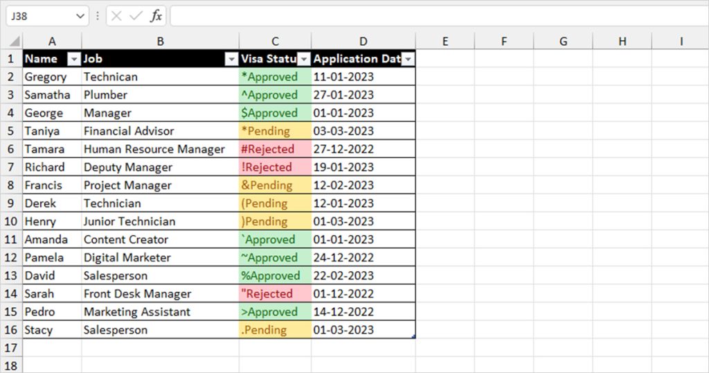
If you take a closer look, you will see that there’s something wrong with the data in column C. Every entry has a special character in front of it. Let’s use the REPLACE function to remove these special characters. First, we create a new column and entered the following formula in cell D2:
=REPLACE($C2, 1, 1, "")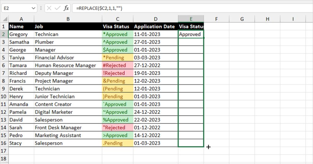
You can see that this removed the first character. Now, apply the same formula to the remaining cells using flash fill. Simply place your cursor on the bottom-right corner of the cell and drag the fill handle.
Use REPLACE to Remove the Last Character
We’re still using the same dataset. Instead, if you now take a look, there are a bunch of different characters, including special characters, numbers, and even text!
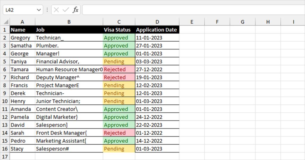
Let’s use the REPLACE function again, but this time to clear the last character in each value of column B. We created a new column and entered the following formula:
=REPLACE(B2,LEN(B2),1,"")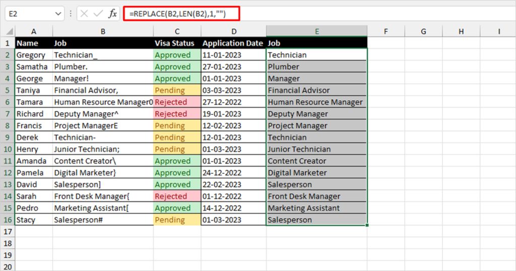
This time, we nested the LEN function. The LEN function returns the character length of the value passed as an argument.
All cells in column B have different character lengths. If we put a specific length to match a specific value, we cannot use Flash Fill to apply the formula in the remaining cells. Let’s take, for instance, we entered the formula keeping cell B2 in mind. Our formula would look like =REPLACE(B2,11,1,"").
Although it would work for B2, when the formula is applied to cell B3, it will not remove the last character because the character length of the value in B3 is 8. The formula will remove nothing.
Use MID
You can extract all values, except for the first, or the last character from the cell using the MID function in Excel. This will basically remove the extra character in whichever position you desire. The MID function is used in the following format while entering the formula:
=MID(text, start_num, num_chars)- text: The cell reference to the content you wish to remove characters from.
- start_num: The text position the function will start looking at values from.
- num_chars: The number of characters you wish to replace from the data.
Remove the First Character Using MID
We will be using a different sheet to extract values using the MID function.
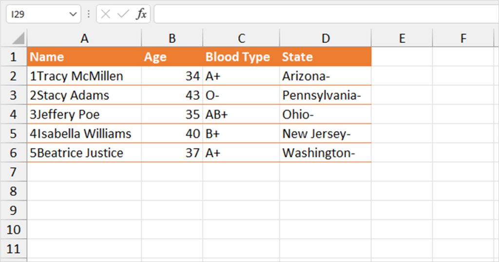
Take a look. In column A, all the names have numbers in front of them. The user probably copies the names, including the number of bullets. You know the drill, we will create a new column and enter the following formula in cell E2:
=MID(A2,2,LEN(A2))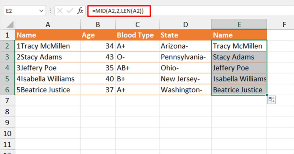
In this formula, the MID function will extract the value from cell A2 beginning from the second position to the length of the cell content. This essentially means that the MID function will extract the value from the second position, ignoring the first character of the value.
Remove the Last Character Using MID
Back to the same table, take a look at column D. It has hyphens that add no value to the overall data.
Let’s modify the MID formula to remove the last character of the data. In our new column E, we entered the following formula in cell E2.
=MID(D2,1,(LEN(D2)-1))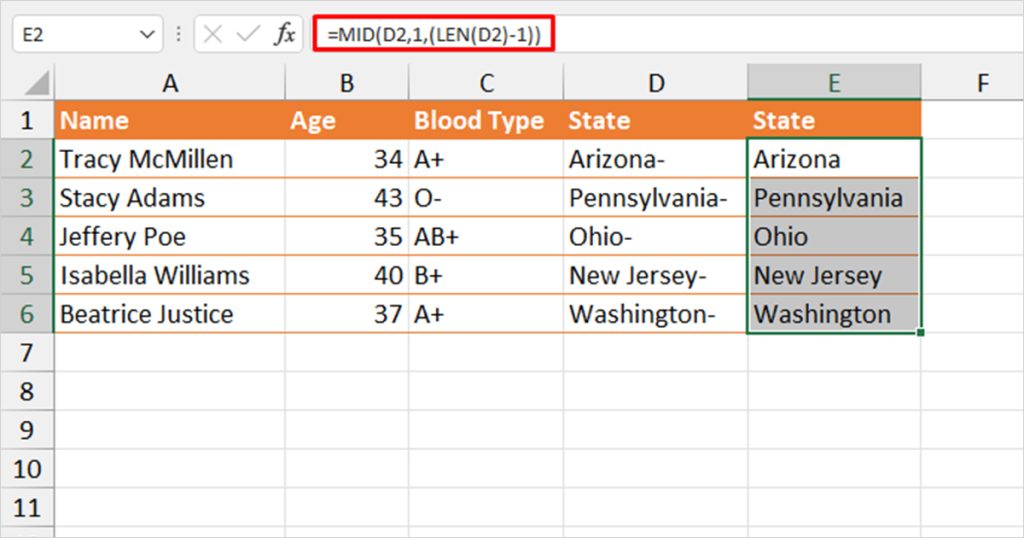
The MID function will extract value from D2 starting from the first position to the second last value of the cell content. This is because we have subtracted one from the total length of D2. For instance, cell D2 has the value “Arizona-”. The total length of this value is 8. When we subtract the value by one, we get the value 7. The MID function will thus only extract 7 values from the first value giving us “Arizona”.
Use the RIGHT Function to Remove the First Character
You can nest the LEN function inside the RIGHT function to create a formula that excludes the first character of a value. Here is what the RIGHT function looks like when written in a formula:
=RIGHT(text, [num_chars])- text: The string you wish to remove characters from
- num_chars: Length you wish to extract
In this spreadsheet, we will be removing the period sign (.) in front of each text in column B.
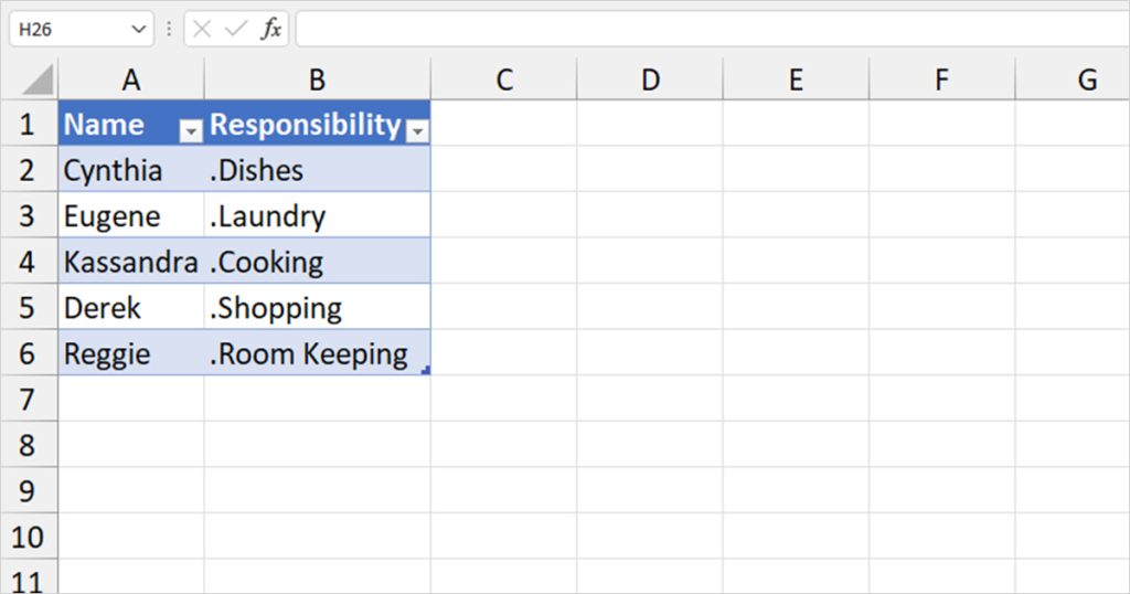
We entered the following formula to remove the first character in cell B2:
=RIGHT(B2,LEN(B2)-1)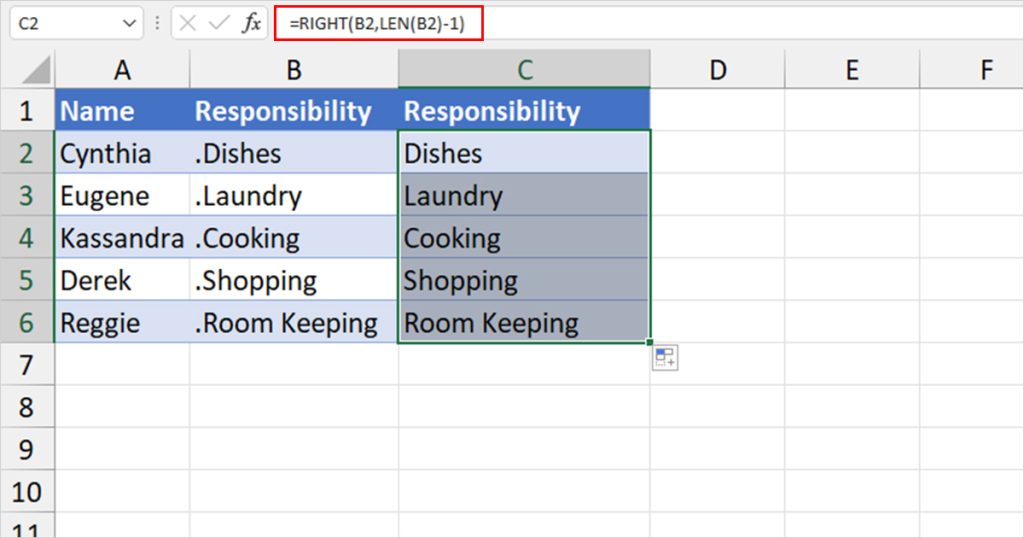
The RIGHT function will extract one less character from the right. This will exclude the first character in the cell content.
Use the LEFT Function to Remove the Last Character
You can use the LEFT function in Excel to extract characters from the left of a value. Here is the format you need to use while entering the LEFT function in a formula:
=LEFT(text, [num_chars])- text: Cell reference
- Num_chars: The number of characters you wish to extract
In this spreadsheet, take a look at column A. Each value has an asterisk symbol after it.
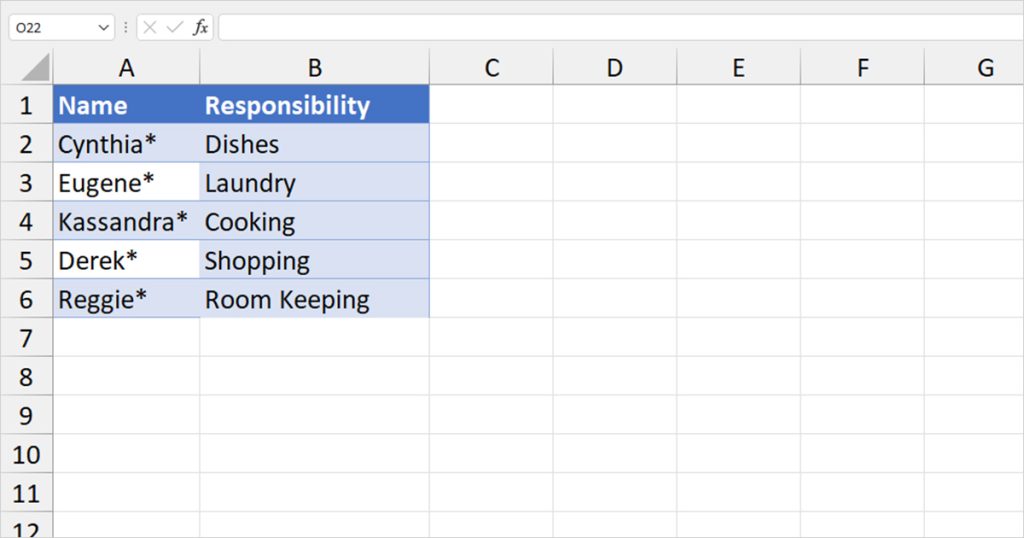
We can use the LEFT function to extract the values that come before the symbol, removing the last character from the value. We entered the following formula in cell C2:
=LEFT(A2, LEN(A2)-1)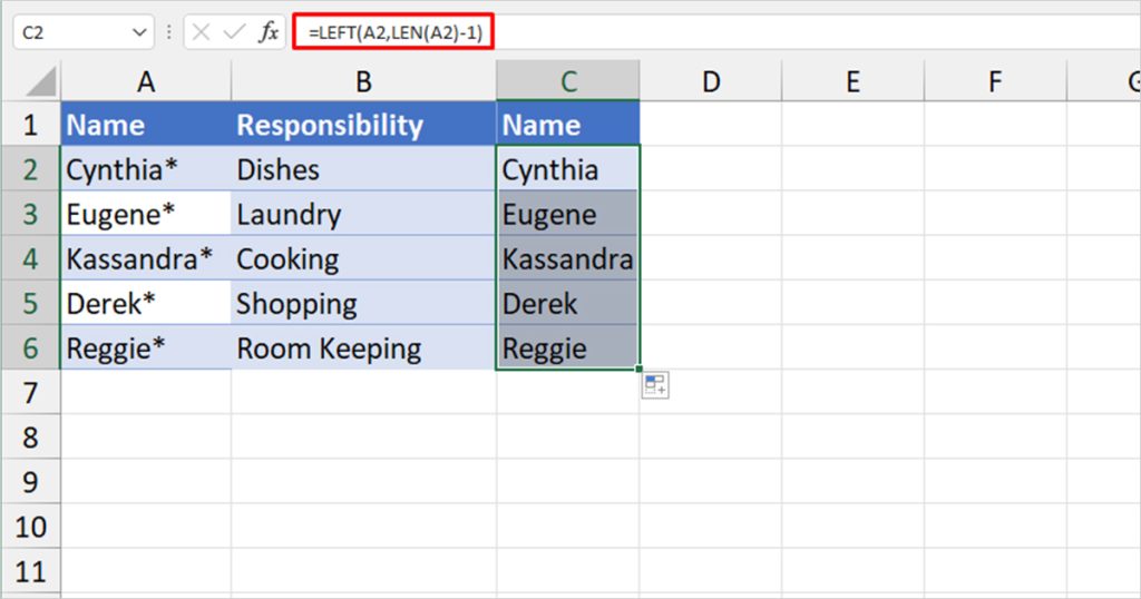
By decreasing the length by 1, the LEFT function excludes the last character from your value. This removed the last character in our data. What we can do now is paste only the values in column C and move our column in place of column B after we delete the column.