In Excel spreadsheets, we barely notice the double spaces in our data. Although these spaces seem insignificant, it can be problematic as Excel takes each space as a character. So, you might not get accurate results while counting the total length of text strings using the LEN function.
Irregular spaces not only mess up the data formatting but also returns errors in calculations. This is why it is best to get rid of such spaces from your data. Here, you can learn how to delete leading, trailing, or all spaces from your values in Excel.
Using TRIM function
Excel’s TRIM function is dedicated to removing all extra spaces from the text. Here, the function will keep only the single spaces in the text. So, you could use the TRIM function for your data to strip away the irrelevant spaces at once.
Syntax: TRIM(text)The TRIM function has only one argument which is text. In this function, you must enclose the value inside quotation marks if you enter a text string. For Instance, =TRIM(“text”). Else, the formula will result in #NAME? error. On the contrary, you do not have to do this for cell references.
Nonetheless, I suggest you use the cell reference as it is easy to input in the formula. Also, after you get results, you could auto-fill the other cells with the Flash-fill handle. Now, without any delay, let’s see the examples of using the TRIM function to delete spaces below.
Suppose, you have a value with spaces in cell A3. To trim the spaces, enter the formula mentioned in the box in a new cell. Create a helper column, if you have data in the next column.
=TRIM(A3)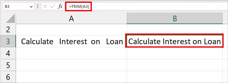
The TRIM function will return the “Calculate Interest on Loan” value as a result. You can see how the formula kept the single spaces while deleting the other spaces. Extend the flash-fill handle if you have more data.
Using Find & Replace
There’s also another way to remove spaces in Excel. You could use this method if you wish to eliminate the spaces directly in the data.
Here, we will use the Find & Replace tool to locate spaces in the text. Then, substitute the space will a null string. This way, the unwanted spaces will be stripped away from your data.
Firstly, select the column with leading spaces and enter Ctrl + H. On Find What, enter Three Spaces and hit Replace All.
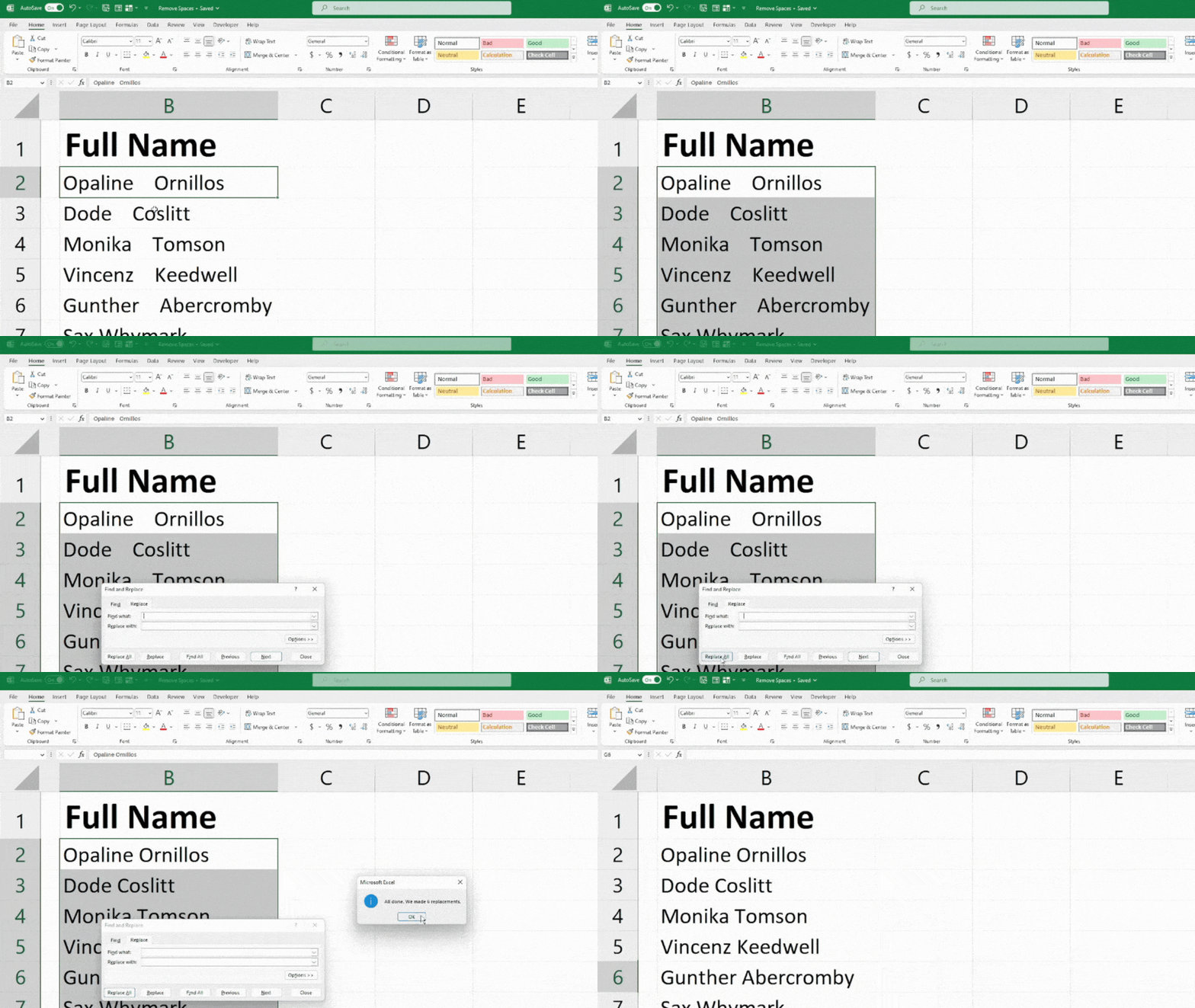
Note that this method will not delete the leading spaces from the value.
Using SUBSTITUTE Function
In the above two methods, we kept the single spaces intact in the texts. But, if you do not want any spaces in your data, this method is for you. We will use Excel’s SUBSTITUTE function to eliminate all spaces.
SUBSTITUTE function returns the replaced value of the old text with the new text. Here, the trick is to replace the value of space with null in the data.
Syntax: SUBSTITUTE(text, old_text, new_text, [instance_num])Before we begin with the application, let us check out the arguments for the SUBSTITUTE function first.
- text: text strings or cell references to substitute values. [Required]
- old_text: the text string you wish to substitute. [Required]
- new_text: new text you wish to substitute in old text. [Required]
- [instance_num]: number of times you wish to replace the old text with a new one. [Optional]
To delete all the spaces of the text in Cell A1, we entered the formula as
=SUBSTITUTE(A2, " ","")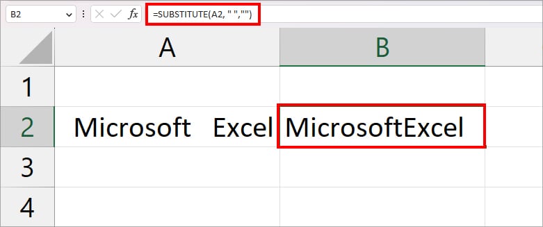
The formula substitutes the “ ” (Space character) of cell A2 with “” (Null string). Then, it returns MicrosoftExcel as an output. With the flash-fill handle, copy down the formula for the other cells.
Rather than texts, I mostly use the SUBSTITUTE function to eliminate the spaces from numbers. For Instance, I have a number with spaces in Column A. But, I want to get rid of spaces to make it a phone number. To do this, I’ll use the same formula with a different cell reference.
=SUBSTITUTE(A5, “ ”, “”)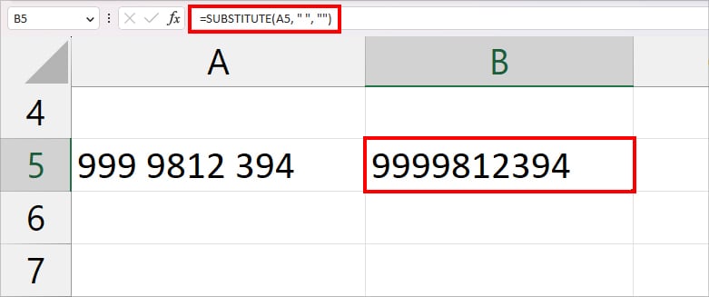
It’ll return 999 9812 394 value as 9999812394.
Using the TRIM and VALUE function
In most cases, you have the trailing spaces in text strings. However, it may persist in number too. When you use the TRIM function, it returns all of the values in text formats. So, while calculating the SUM of numbers with text formats, you’ll get 0 output. That is why we will nest the TRIM function inside the VALUE function.
Let’s suppose, you need to delete spaces in Column A. Now, in a new helper column, enter the formula as
=VALUE(TRIM(A1))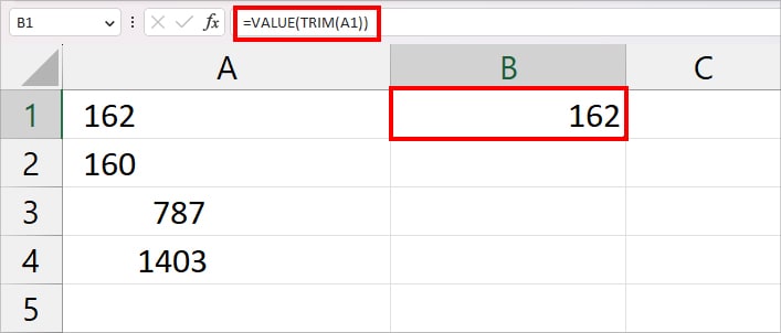
Here, the TRIM(A1) formula will first strip away any unnecessary spaces from the numbers and return the output in text format. Then, the VALUE function changes the output into a number format.