When importing data from external sources, your data may contain redundant values in the form of numbers, texts, special characters, and even hidden characters. Sometimes, these characters follow a pattern such as appearing as the first three characters of your required data.
In cases as such, you can use the REPLACE, LEFT, RIGHT, or MID functions to remove first or last characters. However, in today’s article, we will be using the LEFT and RIGHT functions, along with a VBA code to remove the first 3 characters in Excel.
KEY TAKEAWAYS
- The LEFT function extracts data from the left.
- The RIGHT function extracts data from the right.
- You can create your own function in Excel using the Visual Basics for application language.
How to Remove the First 3 Characters from the Left?
Let’s assume that the data you’re working on has redundant values on the left. We will be using the RIGHT function to remove these characters.
To ensure the formula is dynamic when we apply the formula to the rest of the column, we will next the LEN function inside the RIGHT formula.
Here are the arguments the RIGHT function uses when constructing a formula:
=RIGHT(text,[num_chars])| Argument | Data Type | Description |
text | TEXT | The text or reference you wish to extract data from. |
[num_chars] | INTEGER | The number of characters you wish to extract from the right. |
I have an example to further elaborate on the function’s application. In this sheet, I have data in the range A2:A11. Let’s use RIGHT to remove the first three characters from this data set in range B2:B11.
In cell B2, I entered the following formula:
=RIGHT(A2,LEN(A2)-3)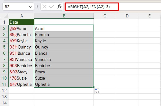
The RIGHT function uses the data in cell A2 as a reference. Then, the LEN function returns the total number of characters in cell A2. In this case, LEN returns 7. After subtracting this value by 3, we get 4 as our num_chars. RIGHT then extracts 4 values from the right, which is “Asmi”.
How to Remove the First 3 Characters from the Right?
If the data you wish to remove from your text is on the right, you will have to use the LEFT function to remove them.
Similar to removing characters from the left, we will be using the LEN function to make our formula dynamic.
The LEFT function uses the following arguments when creating a formula:
=LEFT(text,[num_chars])| Argument | Data Type | Description |
text | TEXT | The source data or cell reference. |
[num_chars] | INTEGER | The number of characters you wish to extract from the left. |
In this sheet, I have data in the range A2:A11. In each data, I have characters on the right I wish to remove. I will be using the LEFT function to extract data from the left, without the unwanted characters on the right.
In cell B2, I entered the following formula:
=LEFT(A2,LEN(A2)-3)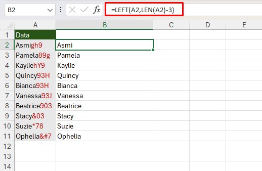
LEFT will use the text in cell A2 to extract data from the left. LEN will return the number of characters in cell A2, which is 7. When subtracting it by 3, it returns 4. Therefore, LEFT will return 4 characters from the left, which is “Asmi”, excluding the three characters on the right.
How to Remove the First 3 Characters from Left and Right?
While you can next the LEFT and RIGHT functions, or even use the MID function to remove three characters from both left and right, they might not be the best approach. This is because using MID would limit you from extracting characters with different character lengths and nesting LEFT and RIGHT would mean a very long formula.
Instead, let’s create a simple VBA code to remove the first three characters from left to right. Make sure you’ve enabled the Developer tab from Excel Options.
We will be using the same functions, LEFT, RIGHT, and LEN to create this formula.
- Go to the Developer tab.
- Select Visual Basic from the Code section.
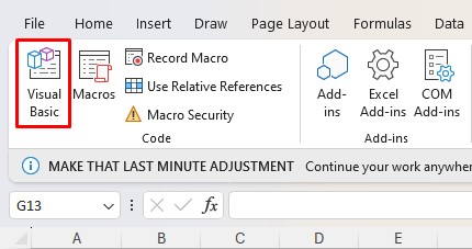
- In the VBA editor window, select Insert > Module.
- In the empty space, copy-paste the following code:
Function Remove_three(text As String) As String
Dim L As String
Dim Final As String
L = Left(text, Len(text) - 3)
Final = Right(L, Len(L) - 3)
Remove_three = Final
End Function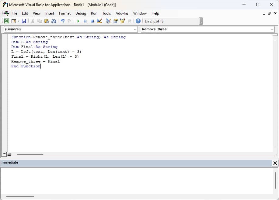
- Head back to your spreadsheet and enter
=Remove_threeon an empty cell.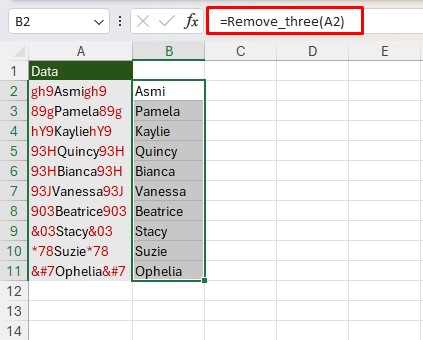
- Enter your text or reference as an argument and hit Enter.
How to Remove Same First Three Characters?
If the characters you’re looking to remove are the same, let’s say 000, then the process of removing these characters is even easier! Excel uses a smart AI to detect patterns in adjacent cells. If you manually remove the first three characters in the adjacent cell, you can use Flash Fill to automatically remove the same characters in the remaining cells!
Here’s an example. In range A2:A11, I have a list of names that start and end with “000”. In cell B2, I manually entered the first data in cell A2, “Asmi”. Now, select range B2:B11 and click Ctrl + E to apply Flash Fill.
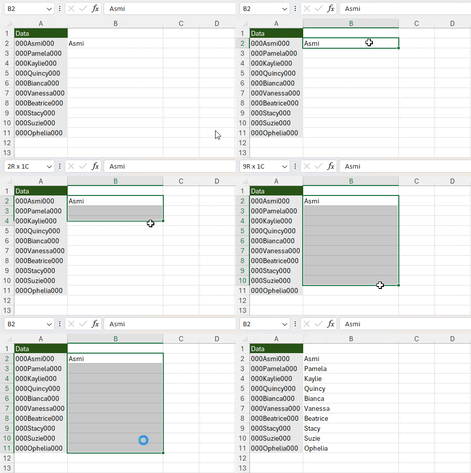
Voila! Flash Fill automatically removes the extra characters from your data.