How to Put a Dash in Excel?

While a dash character is usually treated as the minus sign and used for subtracting numbers, you can insert it as a dash symbol between texts, numbers, or even inside blank cells for various other applications.

For instance, if you have a phone number that looks like 12035550117, it’s difficult to read them without losing focus. 

But, once you chunk it down by inserting some dash signs, the same number 1-202-555-0117, clearly becomes much more readable.

Similarly, you can also put dashes in between text strings and numbers.

Case 1 – Add Dashes in Number 

From Format Cells

Excel’s Format Cell menu has various categories for formatting a number. To insert dashes in Phone numbers or Social Security Numbers, you can apply the Special Format. 

1. Right-click on selected ranges and choose Format Cells.
   
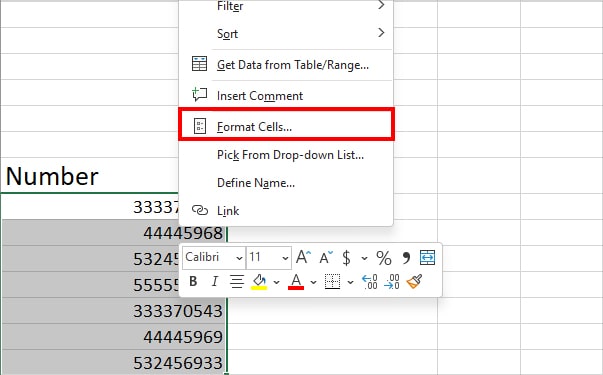
2. On Number Tab, head to the Special menu.
   
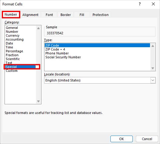
3. Under Type, pick from ZIP Code +4, Phone Number, and Social Security Number to add a dash.
   

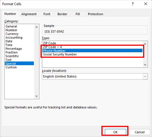
4. Click OK.

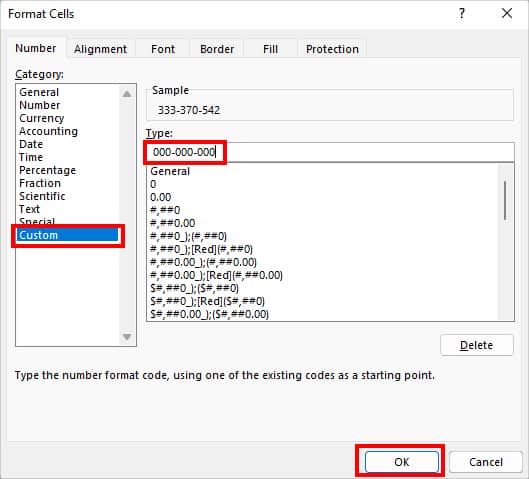
However, if you want to add dashes to numbers in your own way, head to the Custom Format. Under Type, enter 000-000-000. Then, hit OK.

Convert to Accounting Format

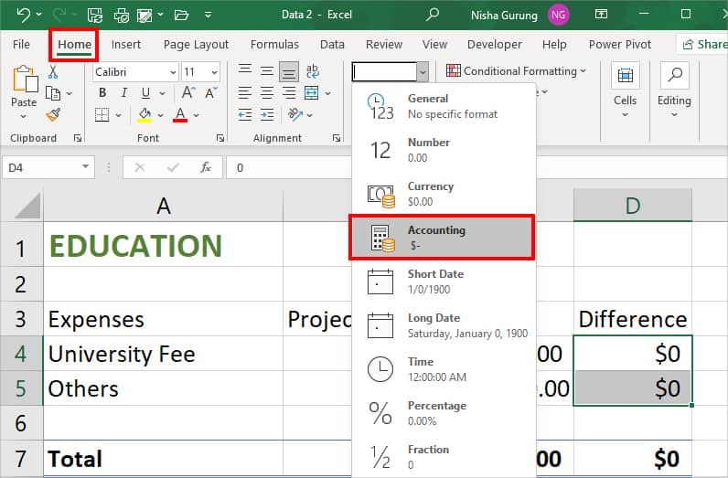
A dash can imply that there is no value in a cell. If you have a 0 value in number data, you could replace them with dashes instead. For this, simply convert the data into Accounting Format. 

Assuming you need to substitute 0 with a dash in the given example, follow the given steps.

1. Select data on your worksheet.
2. On Home tab, navigate to Number group. Then, pick the Accounting format from the drop-down list.
   

From Go To Special

When you have empty cells throughout your Excel worksheet, it can get quite confusing whether they are intentionally left blank or you can fill them with other values. 

To avoid such confusion, it’s better if you fill all the empty cells with dashes. 

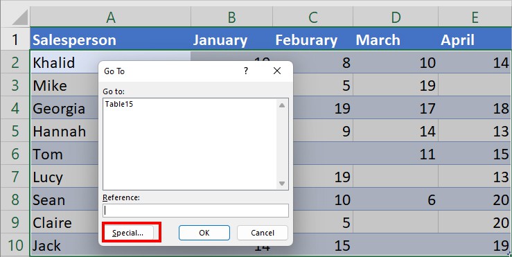
Here, we will first check and highlight all blank cells within the selected range. Then, enter a dash in the selected blank cell. 

1. On your spreadsheet, enter Ctrl + A to select all.
2. Press Ctrl + G to open Go To Window. Click on Special.
   
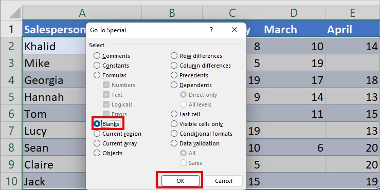
3. Select Blanks and hit OK. (This option selects all Blank Cells)
   
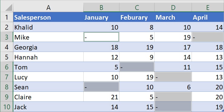
4. Now, type in the (-)  dash character in the first blank cell. Then, hit Ctrl + Enter.
    

Using the Flash fill feature

If you have numbers where you need to insert dashes at specific positions, you can use the Flash Fill. This tool is smart enough to detect a pattern once you enter some values manually. And the good part is that you don’t need to use any complex formula whatsoever.

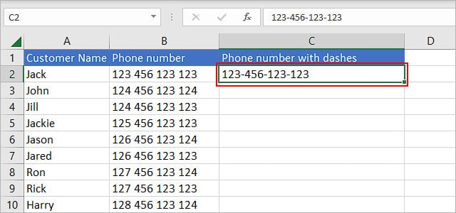
For instance, we have a number such as 123 456 128 903 and we want to insert dashes after every third character so that we get 123-456-128-903 as the output.

1. Create a new helper column to store texts/numbers after inserting the dash symbol.
2. Manually type the first value with dashes at the preferred position and press Enter. Here, we are inserting dashes after every third character.
   
3. Then, start typing the next value. Once Excel autocompletes other cells with dashes, press Enter.
   

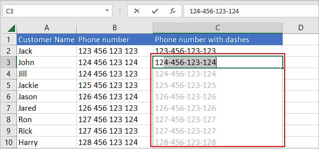
Note: If Excel doesn't suggest the autocomplete list on the second input, type two more values manually and you should get the autocomplete option. Otherwise, press Ctrl + S to save the file and try again.

Using TEXT Function

TEXT Functions are used to modify the formatting of numbers. Using this function, you could apply the Dash format to the values in a cell. It takes two arguments that is value and format. Then, returns the output as text.

Syntax: TEXT(Cell Reference, Format)

Suppose, you need to input a dash in the SSN number. For this, on a new cell, enter the formula as.

=TEXT(C2, “000-00-000”)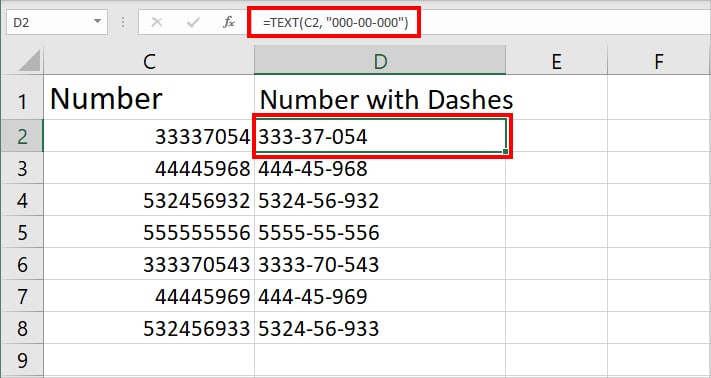 

Here, C2 refers to a cell with a number, and “000-00-000” is the SSN number format to change to. Use the flash-fill icon to have the same format for other cells too.

Using the TEXTJOIN function

If you have a number that’s split into multiple columns, you might want to combine them. However, the & operator and functions like CONCAT simply merge the values without any delimiter.

Luckily, Excel has a function called “TEXTJOIN”, which offers the extra option of adding a preferred delimiter. 

Syntax:=TEXTJOIN(delimiter, ignore_empty_cells, [text])

Where,

• Delimiter: character to insert while joining texts
• ignore_empty_cells: specify whether to accept/reject empty cells while joining texts
• text: cell reference of texts you want to join

For instance,

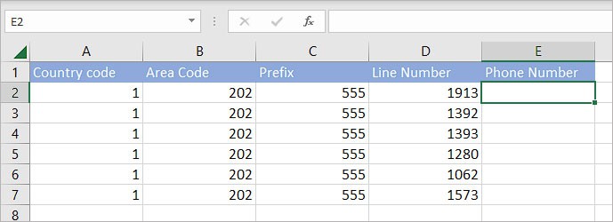
In the above image, we have separate parts of a phone number. But, we want to combine all of them such that we get a complete phone number along with dashes such as 1-202-555-1913.

For this,

1. Create a helper column to store all your combined values and select its first cell.
2. Then, type =TEXTJOIN(“-”, FALSE,.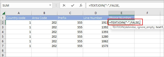
   
3. Now, select the first record containing values you want to combine.
   
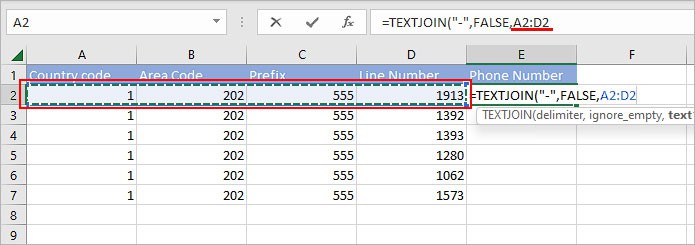
4. Next, complete the formula with a closing round bracket and press Enter.
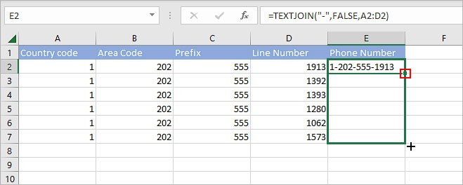
5. Double-click or drag the fill handle to fill other cells with the same type of result.
   

Case 2 – Add Dashes in Text 

From Symbols

Comparatively, Em Dashes are mostly used in Texts than in numbers. If you are fine with manually entering the dashes, you could insert the special character from the Symbols tab. You will have more dashes options like Em Dash, En Dash, Nonbreaking Hyphen, etc. 

1. Launch your worksheet.
2. Go to Insert Tab. Then, from Symbols group, click Symbols.
   
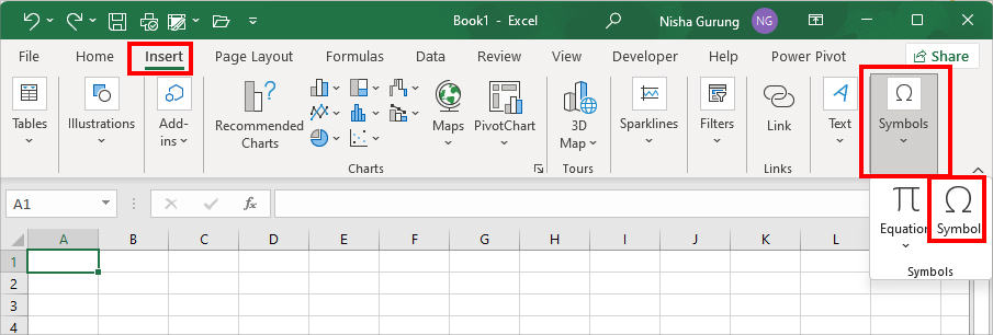
3. On Symbol window, navigate to Special Characters tab.
   
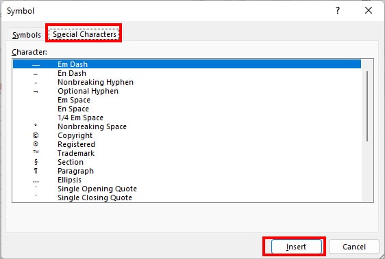
4. From the lists of characters, pick any Dash and hit Insert.

Using Find and Replace

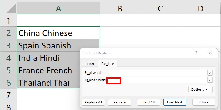
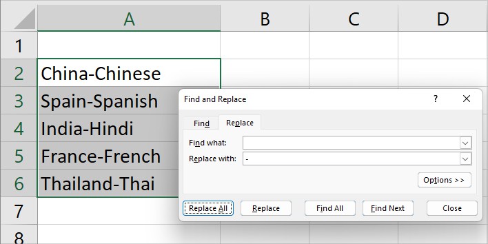
Suppose you need to insert a dash between texts within the same column to separate them. To do so, use Excel’s Find and Replace menu. Here, we will replace the space between the texts with a dash character.

Here’s how you do this.

1. Select data on your spreadsheet.
2. Enter Ctrl + H for Find and Replace Window.
3. On Find What, enter Space. Then, on Replace with, type in a dash – character. 
   
4. Hit Replace All.
   

Using Ampersand Symbol (&)

Another way to insert dashes between texts is by using the Ampersand Symbol. It is mostly used to combine two columns into one. During the process, we will add a dash to return the combined value with dashes. Use this method if you have texts in different columns.

Suppose, you need to join Column A and Column B. Then, add a dash delimiter in between. For this, enter the formula:

=B2&"-"&C2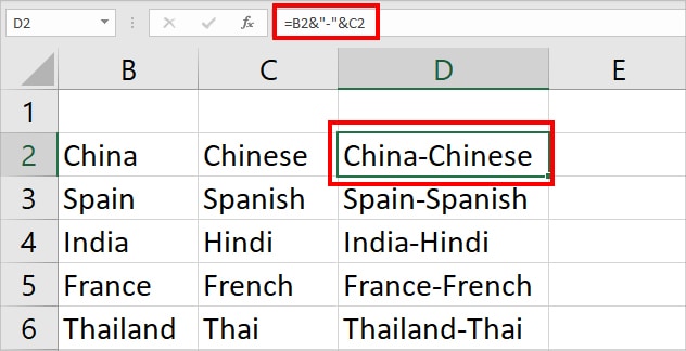 

Using CONCATENATE Function

Similar to the Ampersand Symbol, CONCATENATE Function also returns the combined strings of multiple text strings. You can use this method if you have to combine two or more texts and insert dashes between them. This approach cuts the tedious process of manually entering & symbol every time to join texts for huge text values.

Syntax: CONCATENATE(text1, [text2],...)

To combine Columns A, B, and C while adding a dash sign, enter the given formula in a D cell.

=CONCATENATE(A2, "-",B2, "-", C2)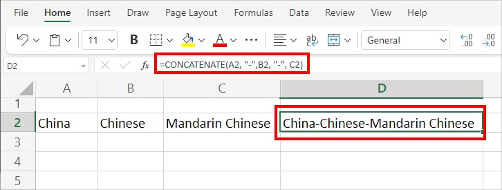

Case 3: Add Dashes in Between Text and Number

There can be instances when you need to add the dashes as delimiters in between the Text strings and Numbers. During such cases, you can use the Power Query Tool to extract the numbers from a text string. Then, using the same CONCATENATE function, we will combine columns and add dashes.

1. Select the Data.
2. From Data tab, click on From Table/Range.
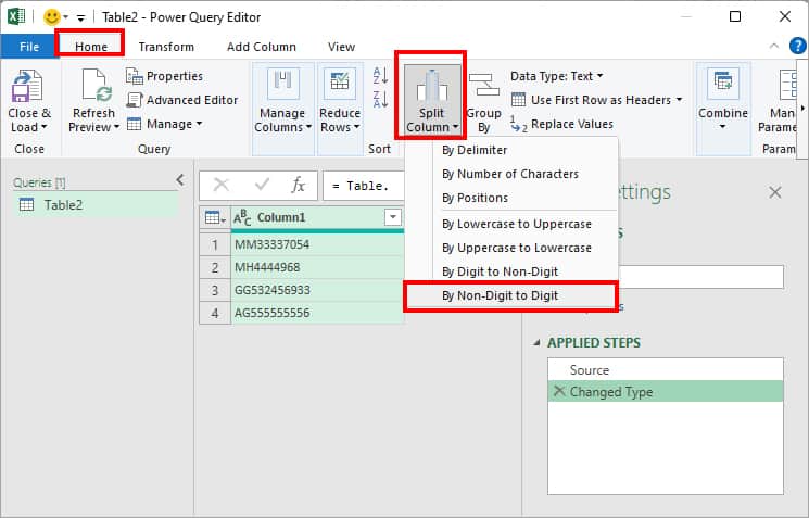
3. On the Home Tab of Power Query Editor, select Split Column > By Non-Digit to Digit. 
   
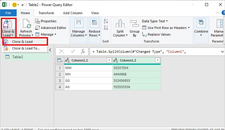
4. Click on Close & Load > Close & Load.
   
5. Now, on Column C2, enter the formula as:
   

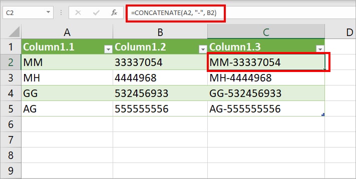
=CONCATENATE(A2, "-", B2)