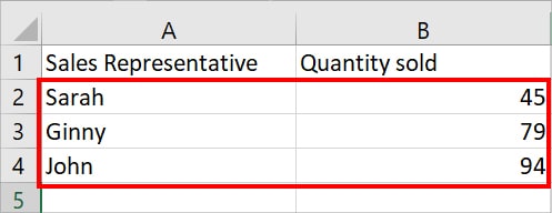
During Excel data entries, it is quite common to have duplicate values. For Instance, you may have two or more students’ names on test mark sheets. While these duplicates are helpful to represent information, they can be redundant and all over the place.
If you find yourself dealing with duplicate values, it is best to merge them and extract only unique ones to declutter your sheet. This will help you to quickly pinpoint any information when required.
Merging Duplicates in Excel means extracting only unique values from the specific ranges. It is similar to removing duplicates but without losing the original information.
You can merge these identical values within sheets or different sheets. Keep reading to learn how to do this in the three cases below.
Case 1: Merge Duplicates Rows and Columns
To merge duplicate rows and columns within the same sheet, we have compiled four methods. Use any method depending on the information you wish to have.
Remove Duplicates
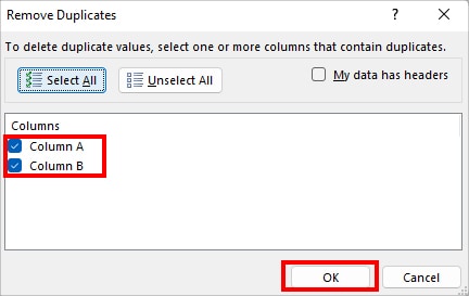
Firstly, you can use the Remove Duplicates menu to merge the row/column duplicates within the sheet. It directly eliminates the identical values and keeps only the unique values.
- On your spreadsheet, highlight cell ranges having duplicates.
- Navigate to the Data Tab. From the Data Tools section, click on Remove Duplicates.

- Under Columns, tick on the Column to filter out the duplicates. Click OK.
Using Filter
The Remove Duplicates menu will permanently delete all identical items from the data. If you want to merge and extract values to another area of the worksheet, use the Filter tool. Here, you can also choose to merge the values in the list itself.
- Firstly, highlight the Ranges on your worksheet.
- Go to Data Tab. Then, from Sort & Filter section, click on the Advanced menu.

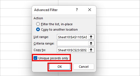
- An Advanced Filter window will pop-up on the screen. Under Action, pick any one option.
- Filter the list, in-place: Select this option to filter out duplicates in the list itself.
- Copy to another location: Choose this option to copy the Unique values in another area. Also, on Copy to menu, select the cell area.
- Tick the box for Unique records only. Click OK.
Using UNIQUE Function
Another method to merge duplicate rows and columns without losing data is by using a UNIQUE Function. Excel’s UNIQUE function discards duplicate values and extracts only unique items from ranges.
Syntax: =UNIQUE(array,[by_col],[exactly_once])Suppose, we need to merge duplicates in the following data. For this enter the formula as mentioned below in a new cell.
=UNIQUE(A2:A19)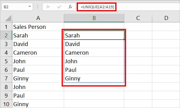
The formula will return only unique names from the data that is Sarah, David, Cameron, John, Paul, and Ginny.
Using Pivot Table
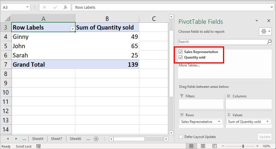
Use this method if you want to merge duplicate items and summarize their value. For Instance, combine all the Sales representative names and calculate the sum of their Total Quantity sold.
- Select the data.
- Go to Insert tab and click on PivotTable.

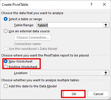
- On Create PivotTable window, choose New Worksheet or Existing Worksheet to import data. Click OK. (If you pick Existing Worksheet, select a new cell reference on Location.)
- On PivotTable Fields at the right panel, check the boxes for the Columns you want to insert.
Case 2: Merge Duplicates Into Single Row
In some instances, you may wish to merge the multiple duplicates into a single row as in the given picture.
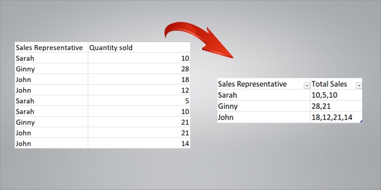
To do so, we will use the Power Query Editor tool to merge columns, transform data, and group all information into one row.
- On your worksheet, select ranges.
- On Data Tab, click on From Table/Range.

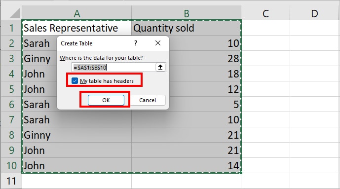
- If prompted, tick the box for My table has headers in the Create Table window. Click OK.
- On Power Query Editor window, select the Column. Go to Transform tab and click on Group By.
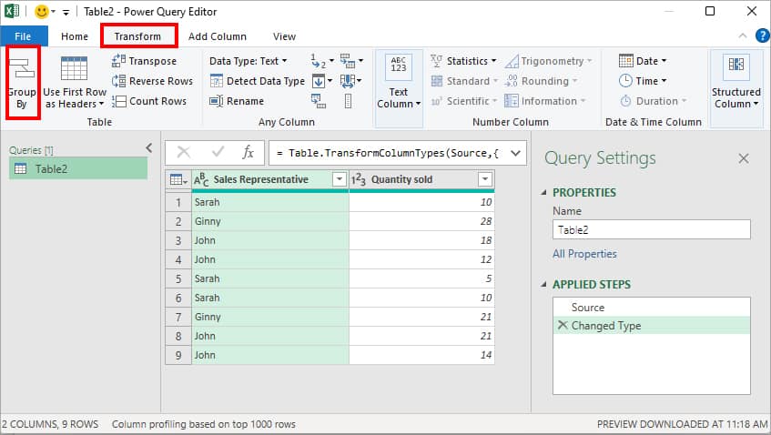
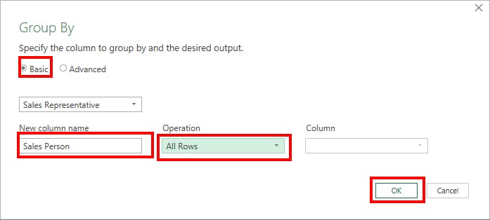
- On Group By window, pick Basic or Advanced option to group columns. Here, we chose Basic.
- Under New column name, enter a name. On Operation, pick All Rows. Then, click OK.
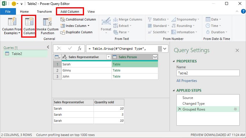
- Now, head to Add Column tab > Custom Column.
- Again, in the New column name field, enter Appropriate name.
- Below Custom column formula, enter the formula as:
Table.Column([Sales Person], "Quantity sold"). (Here, Sales Person is the new grouped column. Quantity Sold is the second column of the Sales Person group. Check the above image for reference)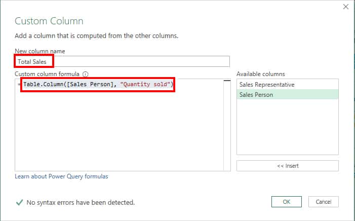
- On a new column, click on Expand icon > Extract Values.
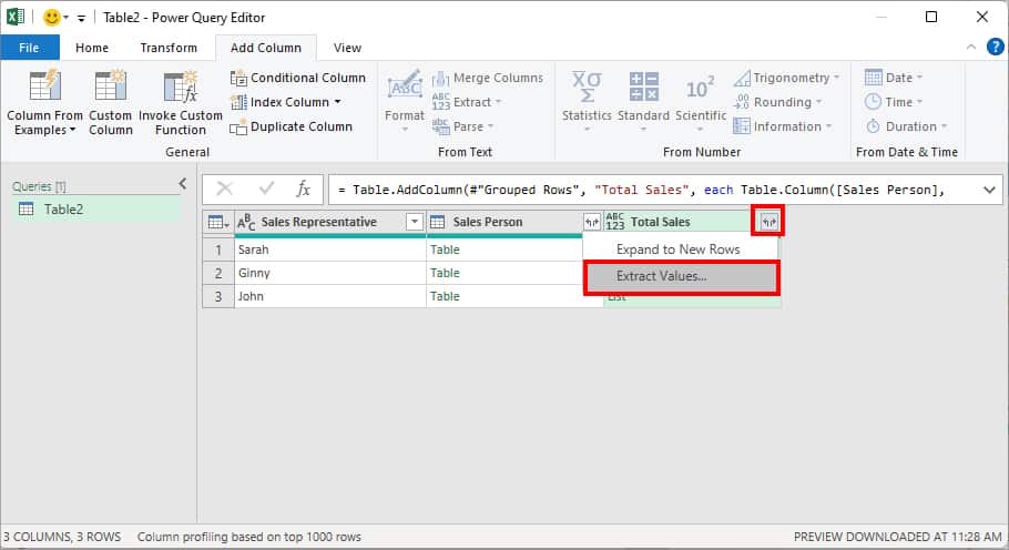
- Pick a Delimiter to separate values in the pop-up and pick OK.

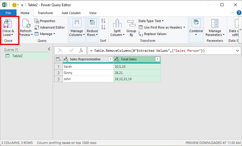
- Now, delete the Middle column. Then, from Home Tab, click Close & Load.
Case 3: Merge Duplicates of Different Sheets
If you have similar data in different worksheets, you can merge the duplicates using the Consolidate tool. With this tool, you can accumulate the value of each sheet and extract them into a new sheet.
- On your workbook, add a New worksheet.
- Click on the Cell to insert merged data.
- From Data Tab, click Consolidate.

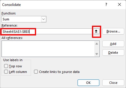
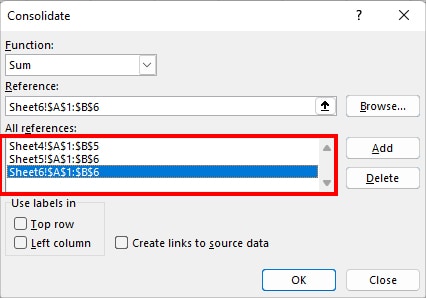
- Now, next to Reference, click on the Collapse icon. Go to a different sheet and select the Cell ranges. Again, select the Collapse icon to exit.
- Now, on All References, click Add.
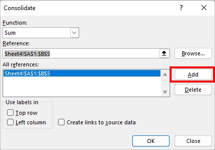
- Repeat Step 4 and Step 5 to add more references from other sheets.
- Below Use labels in, check the box for Top row and Left column. Click OK.
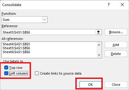
- You’ll have only unique values with the total sum.
