How to Make Negative Number Positive in Excel

You might generate negative numbers when calculating values like profit and loss. While negative values are great indicators of depreciating values, you might want to get rid of them from your sheet. In Excel, you have numerous tools and function to help you automate this task after locating them on your sheet.

How to Make Negative Number Positive in Excel

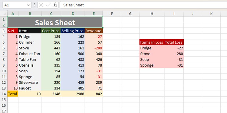
We have a sales sheet in this spreadsheet. There are a total of four items that have a higher selling price in this list of ten items.

We first formatted negative numbers as red, then use the FILTER function in Excel to extract the items with revenue values of less than 0. As we have already labeled these values as loss, there’s no need to keep the negative sign.

We have gathered 7 ways to convert these negative numbers to positive ones in Excel. You can use either of these methods to quickly make this conversion.

Use the ABS Function

The ABS function is a dedicated function in Excel used to convert a number into its absolute value. This means, when you pass a number as a reference in the ABS function, it will ignore the sign used in front of it and generate its absolute number.

Here’s how the ABS function is written in a formula:

=ABS(number)

Let’s use the ABS function to make negative numbers positive in Excel.

On cell J6, we entered the following formula:

=ABS(I6)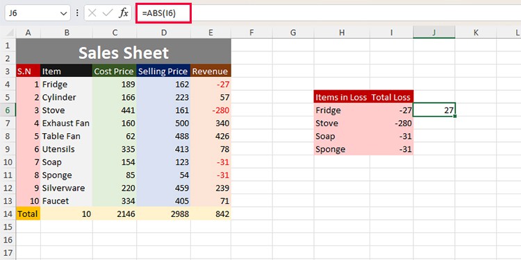

Then, I placed my cursor on the bottom right corner of cell J6 and dragged it to J9. This pastes the formula I applied to the adjacent cells.

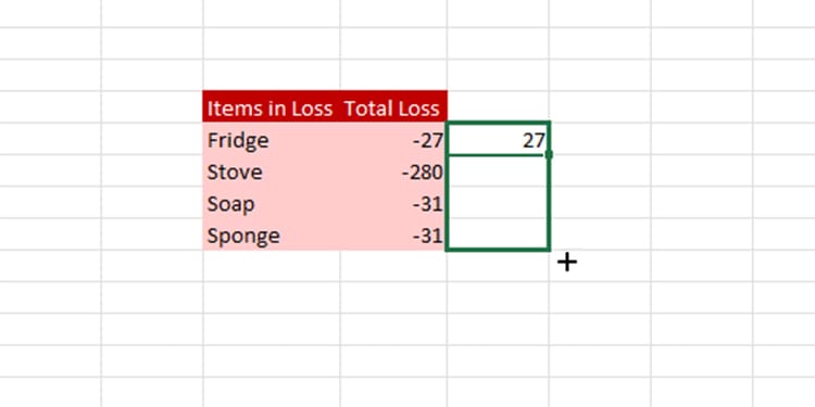
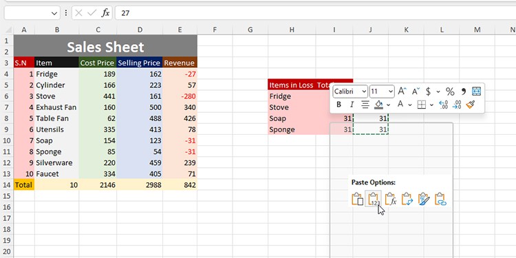
We can now replace our new values with the pre-existing ones in cells I6:I9. However, when you’re pasting your data, make sure to paste these numbers as static values to avoid the #REF error.

Multiply by -1

We know that multiplying anything by -1 returns a positive value. Similarly, the product of a number with one returns the number itself. We can therefore use this logic to make negative numbers positive in Excel.

If you’re trying to convert numbers in a range that does not include negative numbers, you will have to set a criterion. We can use the IF function to only multiply those numbers that are less than 0, which is a negative number.

Here’s the formula I entered in cell J6:

=I6*-1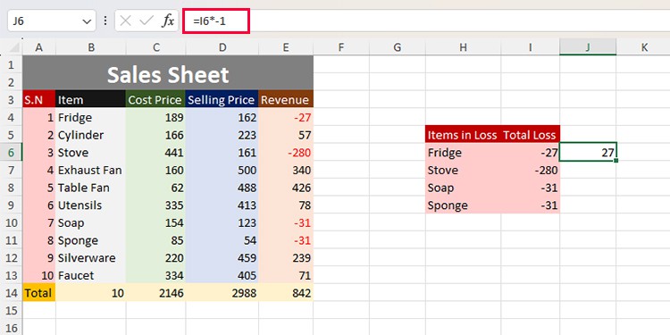

Then, I copied the formula to cell J9 using flash fill.

As I warned you in the method above, always remember to convert the formula into static values before replacing it with the reference value.

Use the AutoFill Feature

We used Excel’s flash fill or autofill feature to paste the above-mentioned formulas into the adjacent cells. However, Excel’s AI is smarter than that. Instead of just pasting the formula, you can also manually convert one number and autofill the remaining numbers.

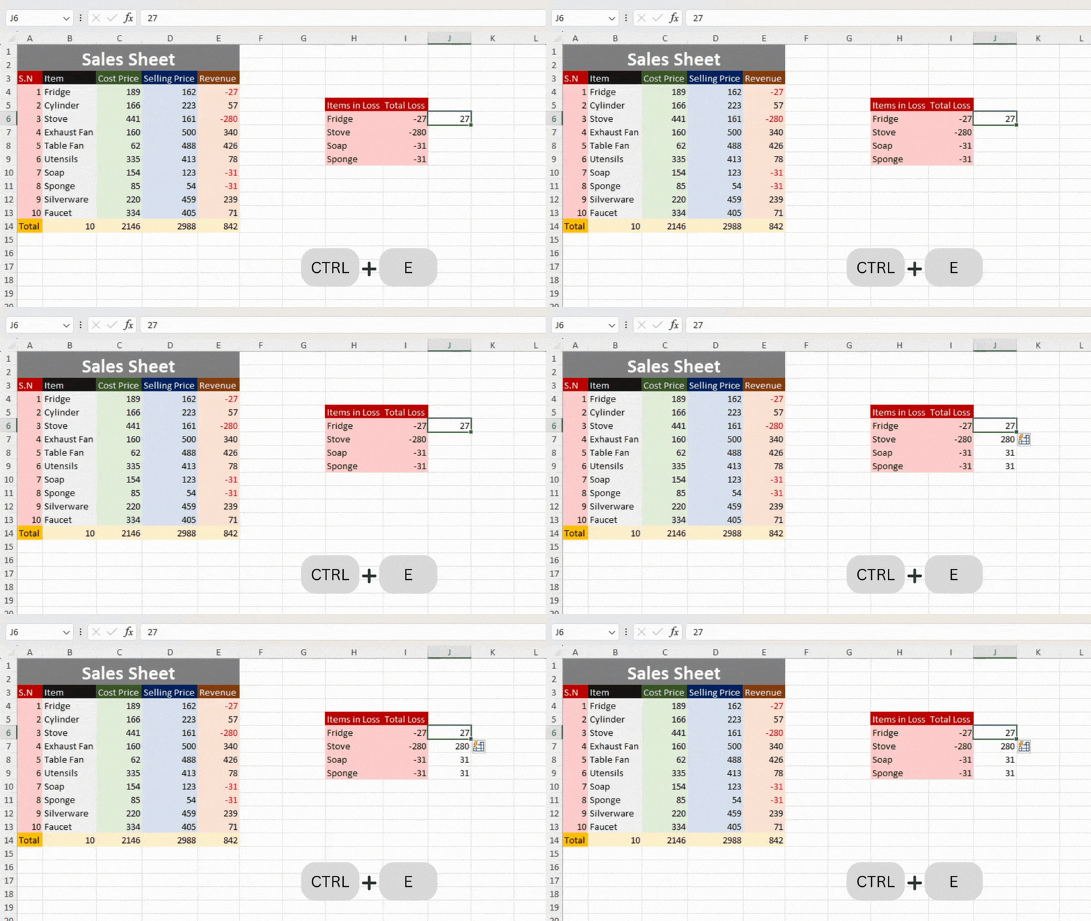
In cell J6, I manually entered 27 which is the first number I wish to convert from range I6:I9. To use autofill, I then used the Ctrl + E shortcut, and voila! Excel’s autofill automatically converted the negative numbers into positive ones. 

Use Paste Special

Using formulas to convert negative to positive numbers includes more than one step. If you’re looking for another method with lesser steps, you can use Paste Special.

However, we cannot use Paste Special in this example. This is because our data in range I6:I9 is part of an array generated using the FILTER function. If I try to use paste special in this range, Excel will trigger the “You cannot change a part of an array” error.

For the sake of this example, let’s change the range into static values. Now, let’s convert these static values into positive numbers using Paste Special.

1. On any random cell, enter -1 and Copy it (Ctrl + C).
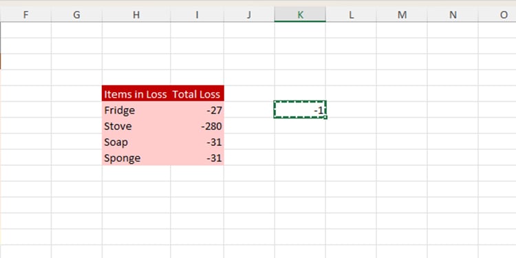
2. Select the range holding the negative values.
3. Right-click and select Paste Special.
   
4. Under Operation, check the box next to Multiply.
   
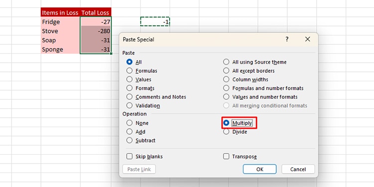
5. Click OK.

Use the Find and Replace Tool

If you wish to change all negative numbers into positive ones on your spreadsheet, this is the perfect method for you. This method is not only easy but also extremely swift. However, if your sheet contains other values, like a formula where you’ve used the – operator, you’re better off using other methods than this as it will remove the – operator from the entire sheet.

1. On your keyboard, use Ctrl + H.
2. Next to Find what, enter -.
   
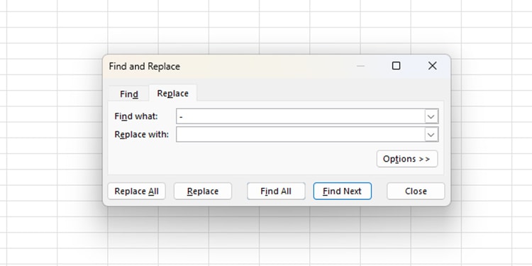
3. Leave the Replace with empty.
4. Click OK.

#NAME? Error After Using Find and Replace?

Notice how I received the #NAME? error instead of a positive number in the range E4:E11, H6, and I6.

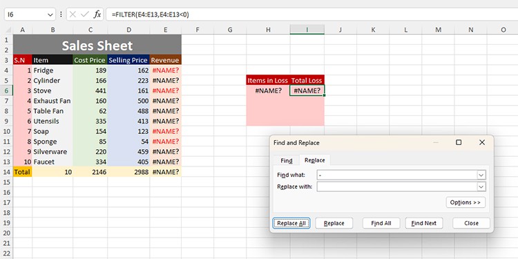
This is because I used the – operator to subtract the corresponding cell in column D from column C. When I removed the operator, the reference changed to something like D4C4, which does not exist, triggering the #NAME? error. 

As both H6 and I6 are dependent on range E4:E14, the error is reflected.

Format Cells Option

You can also change the appearance of your negative numbers into positive from the format cell options. Remember that this change is only limited to the appearance as the number will still behave as a negative number during calculations like subtraction and addition.

1. Select your range with negative numbers.
2. Use the Ctrl + 1 shortcut to open the Format Cells window.
3. Head to Numbers from the sidebar.
4. Under Negative Numbers, choose from two of the options that display your negative number as positive.
   
5. Click OK.

Use Power Query

The Power Query is a powerful automation tool in Excel. You can use Power Query to automate virtually everything on Excel. You can also use the Power Query to convert negative numbers into positive ones in Excel.

1. Select your data range.
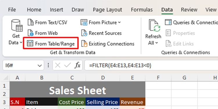
2. Head to the Data tab.
3. From the Get & Transform Data section, select From Table/Range.
   
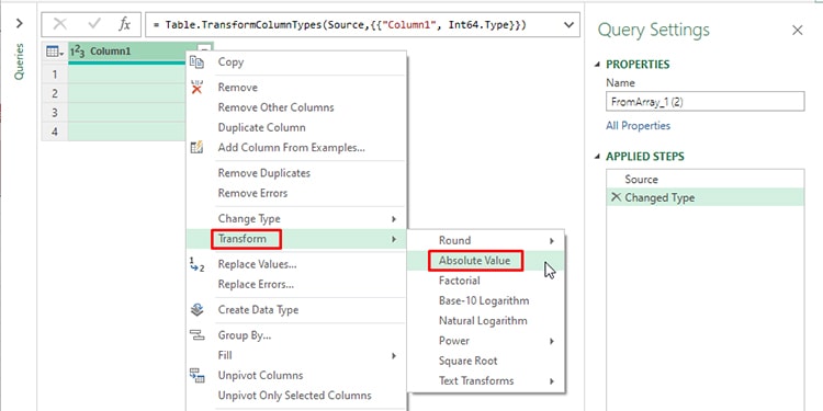
4. Right-click on your column.
5. Head to Transform > Absolute Value.
   
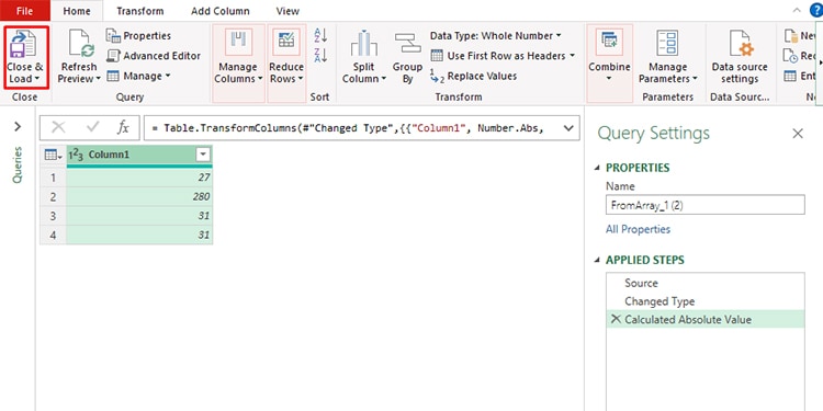
6. From the Home tab, click Close & Load.