How to Make Decision Tree in Excel

If you’re having a hard time deciding on something, you could create a Decision tree in Excel. For Instance, it could be a conclusion regarding the house purchase, product budget, and many more.

A decision tree analyzes all the possibilities and uncertain outcomes of the main decision. So, it helps you make the best choices for personal or professional purposes. In Excel, there are two different ways to make a decision tree.

What Are the Elements Used in a Decision Tree?

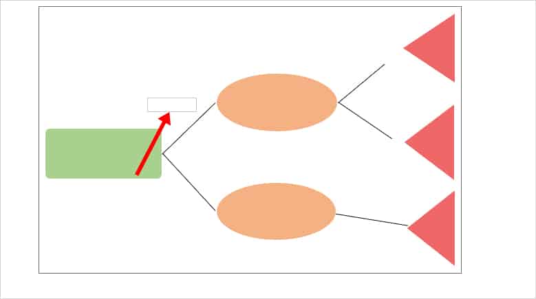
A decision tree comprises four different nodes such as the decision node, chance node, branches, and end notes. Before you plot the decision tree, you must understand what each node refers to. This way you won’t have any confusion creating the tree.

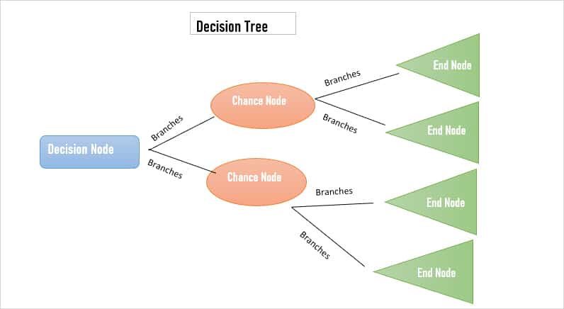
• Decision Node: It portrays the main decision in a diagram. You could create a rectangle shape for the decision node.
• Chance Node: It illustrates the probability or uncertain results of the main decision. Usually, there are two chance nodes in the decision tree. You could represent the chance node with a circle shape.
• Branches: Branches represent the potential outcome.  
• End Node: It shows the final outcome of the decision. In most cases, users illustrate the end node with a Triangle shape.

How to Make Decision Tree in Excel?

In Excel, there are three different ways you can make a decision tree. You could draw each basic shape such as Rectangle, Circle, or Triangle for the nodes. Or, you could opt for SmartArt if you want to quickly create a tree. 

Using Basic Shapes

Excel has all types of shapes such as Basic, Rectangles, Block Arrows, flowcharts, Callouts, and many more. You could insert these shapes to create a decision tree for your data in Excel. This method is beginner-friendly as well as flexible. You can choose your preferred shape for the decision tree. 

Here, we will be using basic shapes like rectangles, circles, and triangles to create the original decision tree. 

Step 1: Add Decision Node

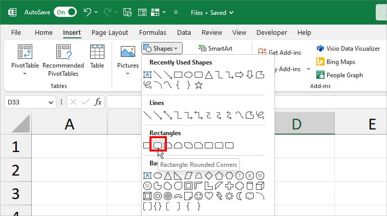
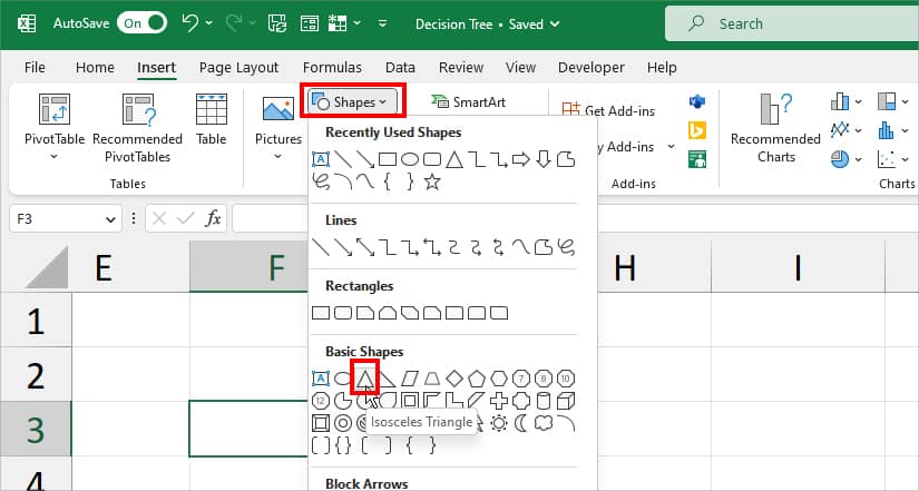
1. On your worksheet, go to Insert Tab.
   
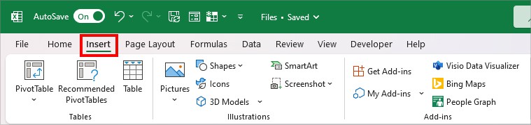
2. From the Illustrations section, click on Shapes menu.
   
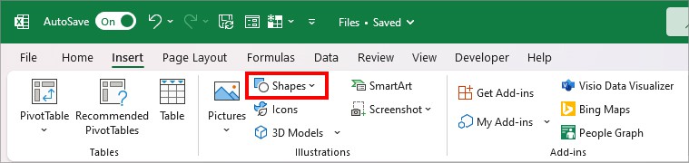
3. Then, pick a Rectangle Rounded Corners shape for the Decision Node. Using the Plus cursor, draw it on your sheet.
   
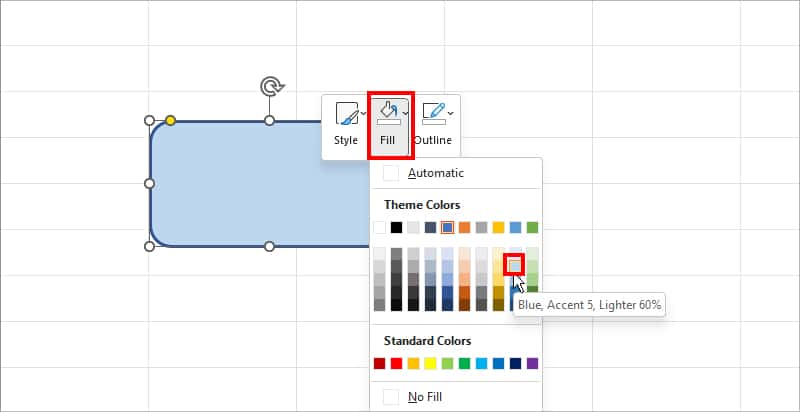
4. Resize the rectangle shape as needed. Then, while the shape is still selected, right-click on it. Expand the Fill icon and pick a different Colour.
   
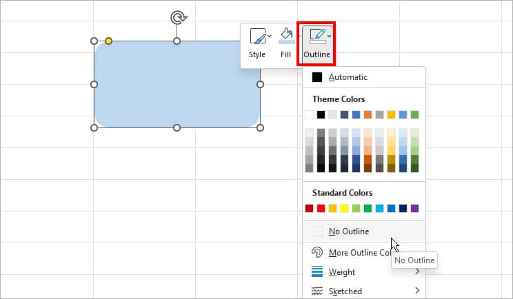
5. Again, right-click on the Shape and click on Outline. Then, select a Color or No outline for your shape.
   

Step 2: Add Chance Node

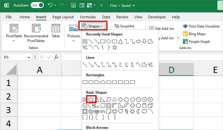
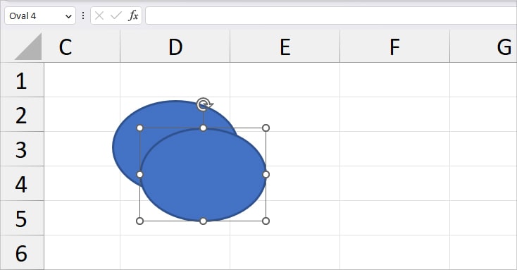
1. Head to the Shapes icon and choose an Oval shape for the Chance Node. Draw a Circle shape on your sheet. 
   
2. Adjust the Circle size as required. 
3. Then, while the circle is still selected enter Ctrl + D keys together. You’ll have another Circle of the same size.
   
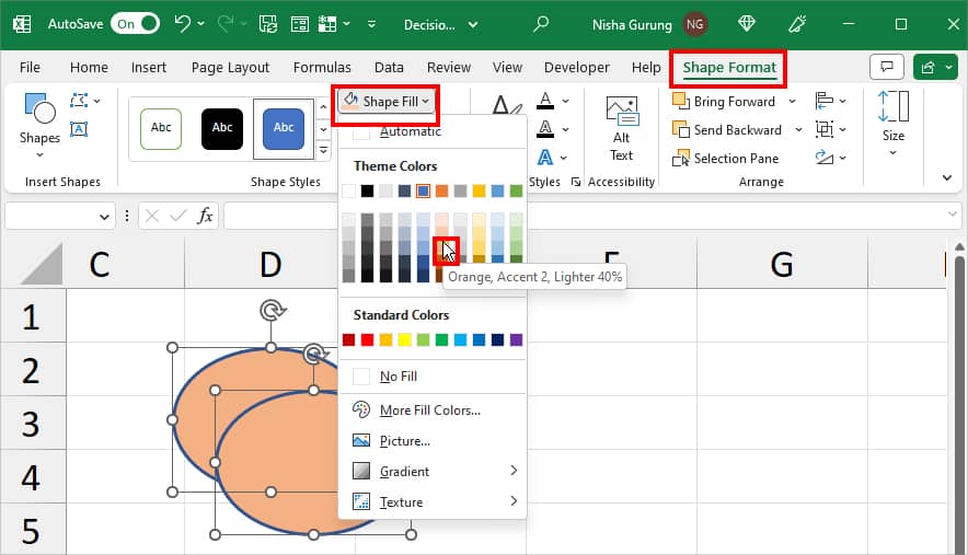
4. Select both circles and head to the Shape Format tab. From the Shape Styles section, expand Shape Fill and choose a different Colour.
   
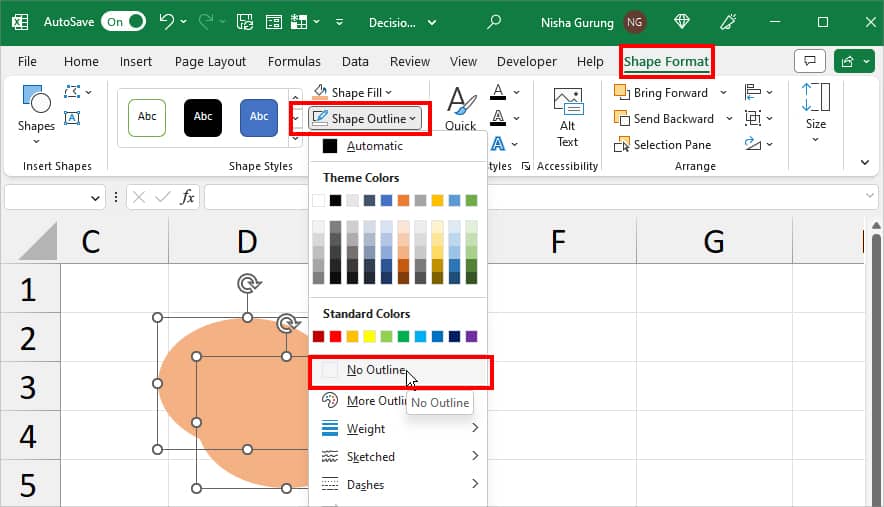
5. Again, click on Shape Outline. Pick a Border style and Color for your circle. Then, change the circle position such that it illustrates two Chance Nodes.
   

Step 3: Add End Node

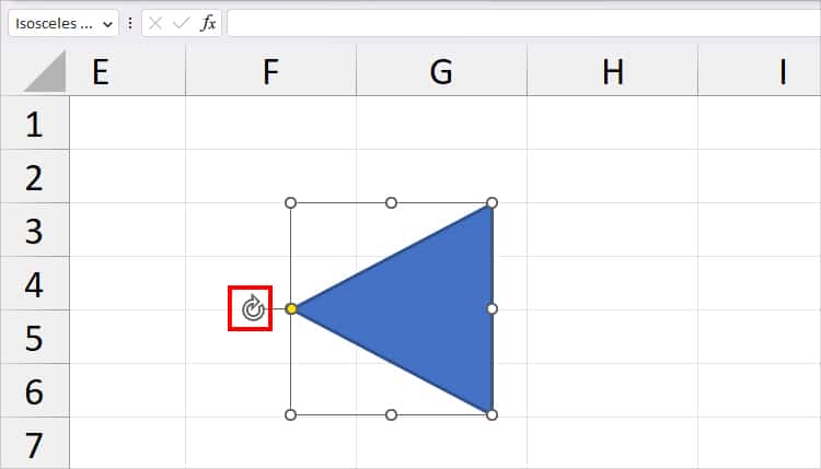
1. From the Shapes icon, choose a Triangle Shape for your End node and draw the shape on your sheet.
   
2. Using the Rotate Cursor, rotate the Triangle towards the left.
   
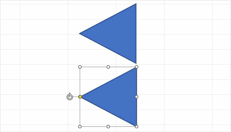
3. Again, to have one more End Node, press down the Ctrl + D keys while the triangle is still selected. Re-position the Triangle.
   
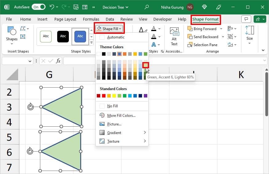
4. Now, select both End Nodes and fill in a different color from the Shape Format Tab.
   

Step 4: Add Branches

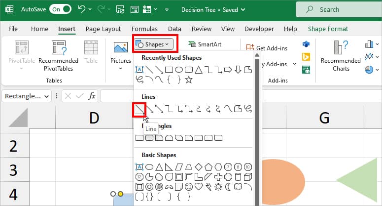
1. Finally, from the Shapes icon, choose a Line shape. Then, draw a Line to connect the Decision Node to Chance Node.
   
2. Again, draw another Line on your sheet. Reposition the line such that it forms a < shape. 
   
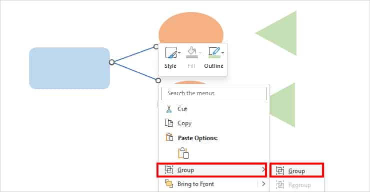
3. Select both Lines and right-click on them. Pick Group > Group from the context menu.
    
4. Now, select the line and enter Ctrl + D to duplicate them. You could use the duplicate line shape to connect the Chance Node with End Node.
   
5. You can draw extra shapes for Chance or End Nodes if needed.

Step 5: Insert Probabilities and Outcomes Into the Shapes

Now, we have a shape outline of the decision tree. In this final step, we will add data and format the texts to complete the decision tree. 

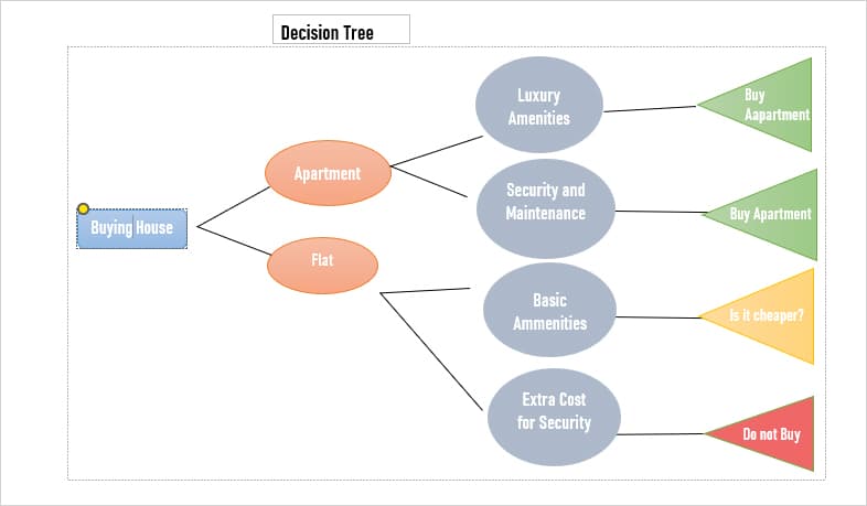
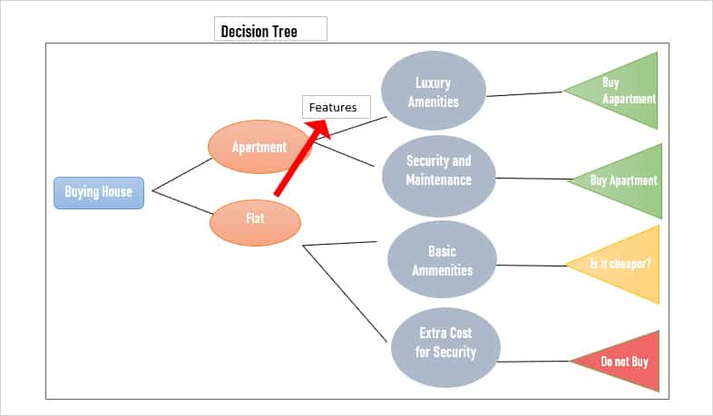
Example: Sam has a confusion about his housing decision. According to him, there are two possible chances to buy .i.e. a flat and an apartment. Now, for this, he needs to look after his budget and the features. Let us see how he can decide which house is best for him.

1. Double-click on the Decision Tree box. When the cursor appears, start typing in your information. In our case, Buying house is the Main Decision.
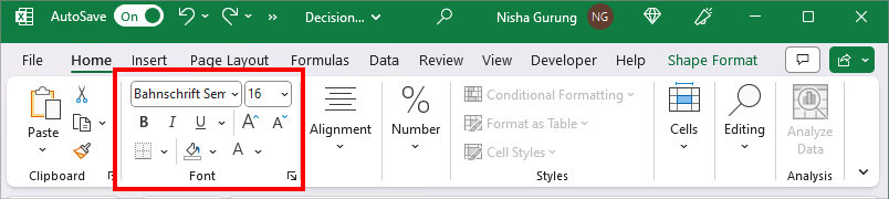
2. Select the entire Text. Then, from the Font section of the Home Tab, change the Font Style, Colour, and Font size as per your preference.
   
3. Repeat steps 1 and 2 for Chance Node and End Node. Here, Apartment and Flat will be the first Chance Node. Then, again, features will be second-chance nodes. End Nodes will be the decision whether to buy house or not.
   
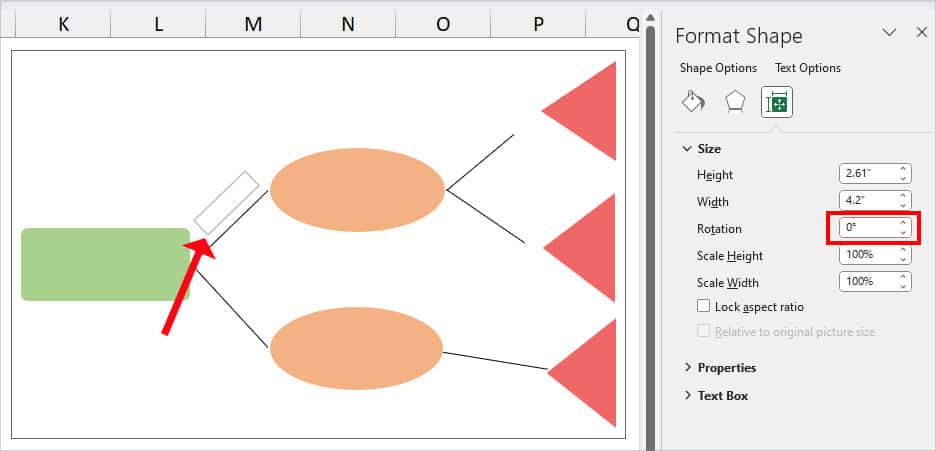
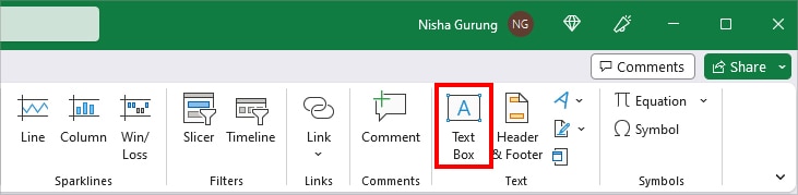
4. Now, to input the information in the Branches, head to Insert Tab and click on Text Box.
   
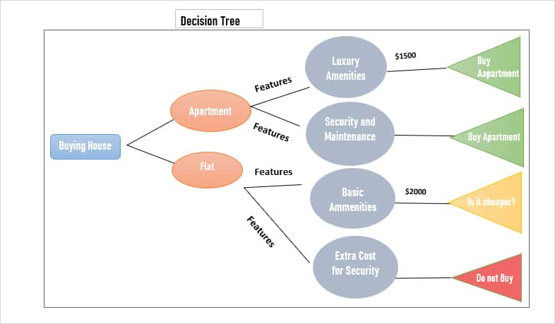
5. Draw a Text box and place it right above the branches. Then, enter Data in the Text box. 
   
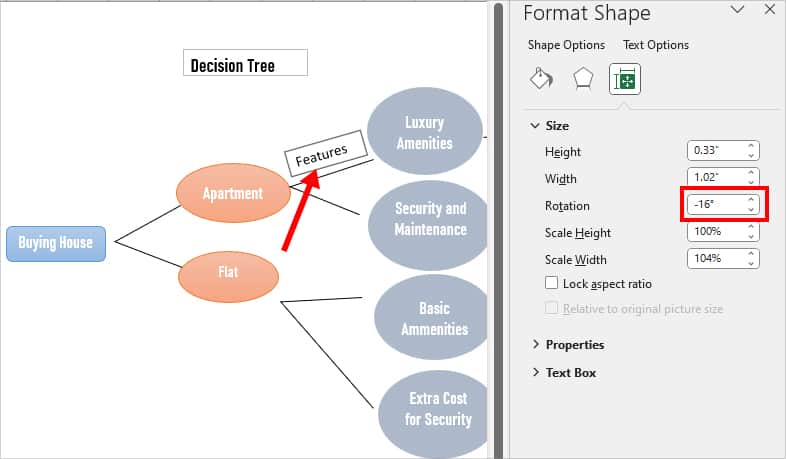
6. Select the Text box. Then, from the Shape Format tab, expand the Size menu. Slightly Rotate the box by increasing or decreasing the Rotation menu. Make sure it appears in the angle counterclockwise direction.
    
7. Repeat step 6 for all the other branches. Then, rotate the textbox towards the right for the Second Chance and End Nodes.
   

Using SmartArt

If you feel like manually drawing shapes and creating a decision tree is extremely time-consuming, we have another alternative for you. In this method, we will use Excel’s built-in Horizontal Hierarchy SmartArt Design to shorten the process. 

This design has connecting lines and rectangle shapes which is perfect for a decision tree. You could leave the rectangle shape for Chance and End Nodes as it is or change the shape. Also, the design already has a text format in each shape.

Step 1: Insert Horizontal Hierarchy Design

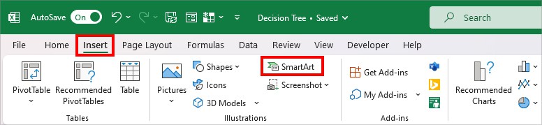
1. On your Worksheet, go to the Insert tab.
2. From the illustrations group, click on SmartArt.
   
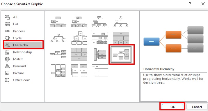
3. On the SmartArt Graphic window, head to the Hierarchy category and pick Horizontal Hierarchy design. Hit OK to confirm.
   

Step 2: Format Shapes 

This step is completely optional. You can skip this and directly edit the texts if you want.

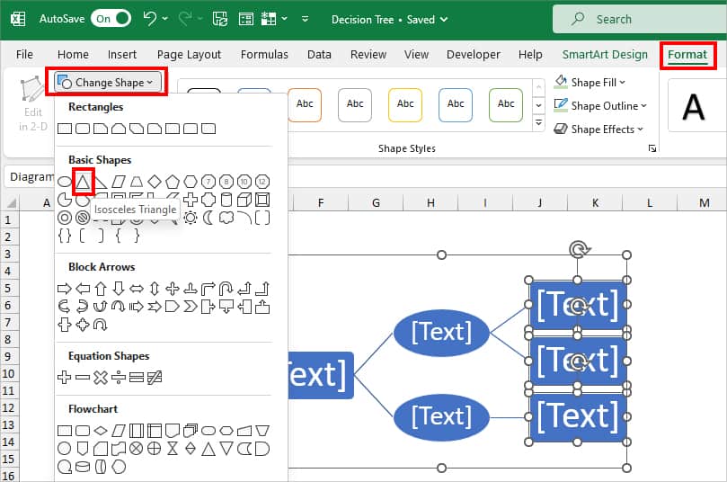
1. Firstly, select the Two Rectangles of the second part and head to the Format Tab. From the Shapes group, expand the Change Shape Menu and click on Oval Shape.
   
2. Now, select the other Three Rectangles at the end and go to the Format tab. Click on Change shape and pick a Triangle shape.
   
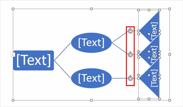
3. Select all Triangle shapes and rotate the Triangle towards the left. Note that as all the shapes are grouped, you must be careful while selecting the triangle.
   
4. Resize the Triangle shapes if needed.
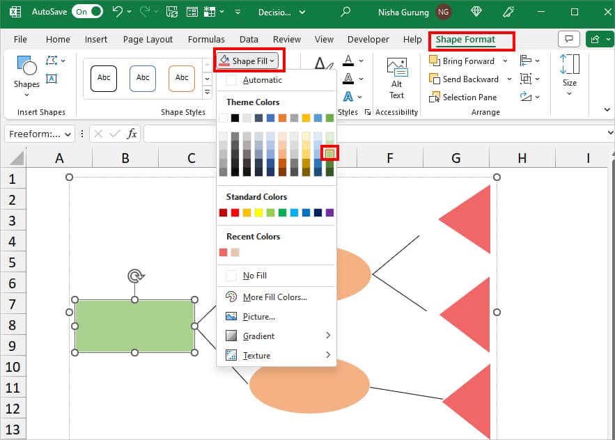
5. To change the shape color, select a Shape and go to Format Tab. Expand the Shape Fill and pick a different color.
   

Now, you can input the Decision Node in the rectangle box, Chance Node in Circle, and End Node information in the triangle just like above. After typing all the required information, you can change the Font format, Style, Size, and Color.

Step 4: Add Text Box

To add information in the Branches, you need to add an extra text box. Unlike other shapes, you cannot edit texts in the lines.

1. From the Insert Tab, click on Text Box.
   
2. Draw a Text box right above the branches. Type in the information inside the box and format the font.
   
3. Select the Text box. Then, from the Shape Format Tab, expand the Size icon. On the Rotation menu, increase or decrease the button to rotate it towards the left.