How to Make a Box in Excel

If you’re starting out in Excel, learning smart tips and tricks can help you use the application like a professional. Making a box in your spreadsheet is definitely one of them. Excel has different types of boxes like Textbox, Checkbox, List box, Search box, etc you could use for respective purposes. 

For Example, an in-built Checkbox form can be beneficial in creating a checklist. Similarly, you could customize your cell and make it a Search box to quickly pinpoint any information. Nonetheless, today, we will guide you through the steps to insert all types of useful boxes in Excel.

Text Box

If you’re adding a long paragraph in Excel, you can insert a Textbox to easily fit everything. While the Wrap Text feature can do the work, I prefer Text Box over it to avoid resizing other cells. Besides, these text boxes can be also useful to enter supporting information or descriptions anywhere on your sheet. For Instance, you could add them to your Charts and figures too. 

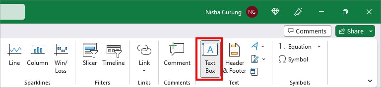
1. On your sheet, head to Insert Tab. 
2. From the Text group, click on Text Box.
   
3. Draw a Text Box of your preferred size using the cursor.
   
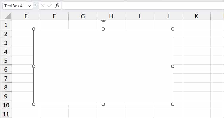
4. Click on the Box and start typing the text.
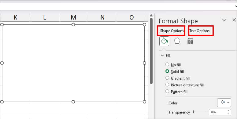
5. To format the text box, right-click on the box and pick Format Shape.
   
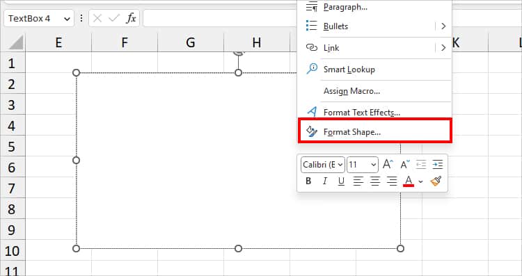
6. Explore all options of both Shape Options and Text Options. Then, customize the box as you wish.
   

List Box

In Excel, you can create a List Box to present a list of information. Here, when you represent the list in a box, users can actually pick a value. Also, the value you choose is reflected in the linked cell. Meaning, you can see the number position of the value in the cell.

Excel has a default List box menu in the Developer Tab. If you cannot see it in the Ribbon, you would have to add the Developer Tab first. But, users who already have the Developer tab in the Excel Ribbon can skip Step 1. 

Step 1: Add Developer Tab

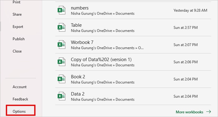
1. Launch Excel and go to the Options menu at the bottom left.
   
2. On Excel Options window, head to Customize Ribbon category. Below the Main Tabs, tick the box for Developer. 
   
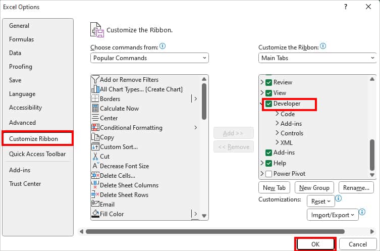
3. Hit OK.

Step 2: Create List Box

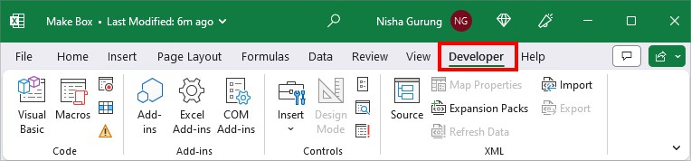
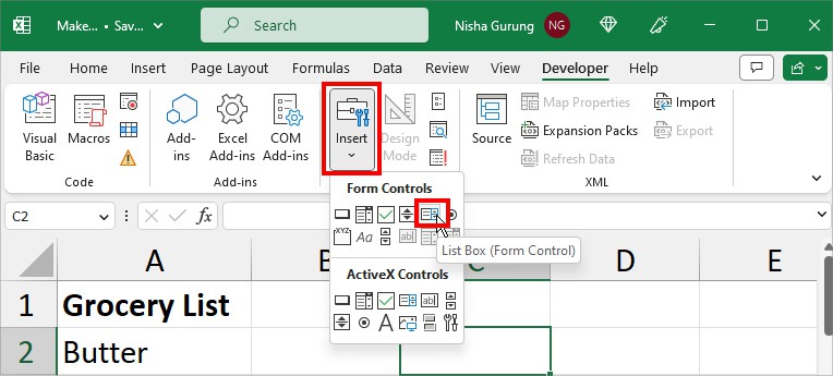
1. On your Sheet, go to Developer Tab.
   
2. From the Controls section, click on Insert > List Box. 
   
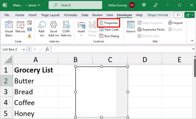
3. While the box is still selected, click on Properties from the same Controls group. 
   
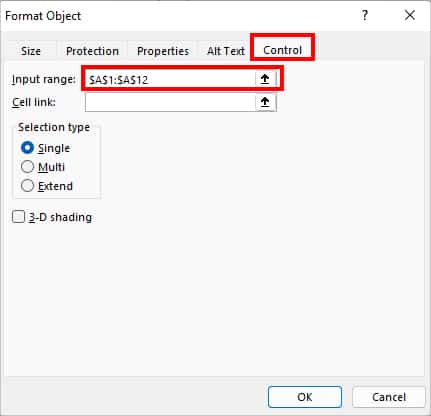
4. On Format Control, head to the Control tab. Then, on the Input range, select the cell ranges containing Lists with the Collapse icon.
    
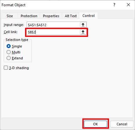
5. On Cell Link, select an Empty cell to create a reference link and hit OK. Note that this cell will display the numeric position of the value when you click on any information from the list.
   
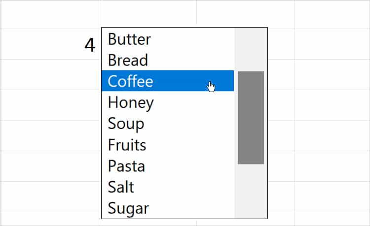
6. When you select an item from the list box, the number will appear in the linked cell. Here, Coffee is in the fourth position in the list box.
   

Check Box

When it comes to creating a checklist, Excel’s checkbox features are the best. These checkboxes are clickable which makes it easier to tick off the completed lists. As it is an in-built form, you do not have to manually create rectangles and insert tick marks for the checklists. 

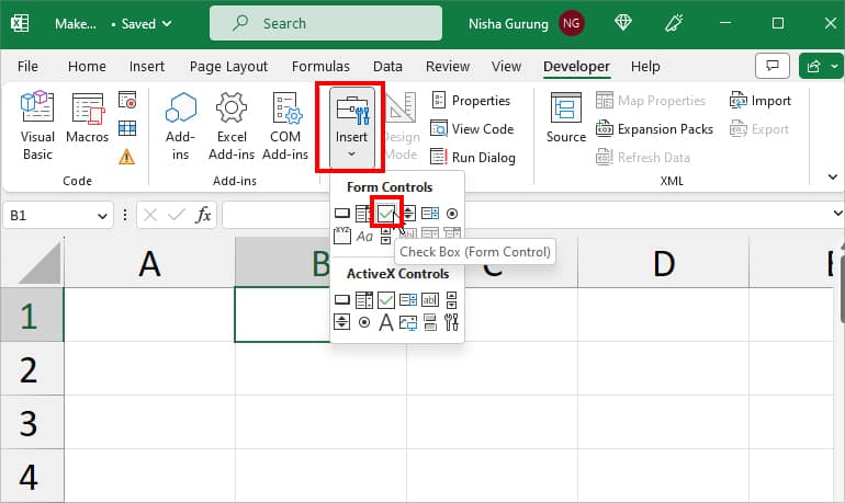
1. On your Excel Sheet, go to the Developer Tab.
   
2. From Controls section, click on Insert. Under Form Controls menu, click on Check Box.
   
3. Click on a Cell to add the Checkbox. 
   
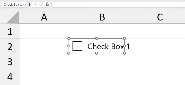
4. Select the Check box and Rename the list.
5. Repeat the steps to make multiple checkboxes. Then, simply click on the Box to tick it.
   

Search Box

Locating the exact information in the massive records can be quite a hassle task. But, you can create a Search box to easily locate the desired information from your data. Not only will you be able to locate but also highlight the information to make them easily stand out in the sheet. 

To create a Search Box, we will use Excel’s conditional formatting. Here, we will set a rule for one of the empty cells in the spreadsheet to make it function as a Search box.

1. Firstly, select all data on your spreadsheet.
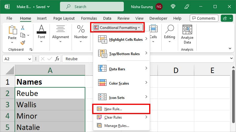
2. From the Home tab, click on Conditional Formatting in the Style section. Then, pick New Rule.
   
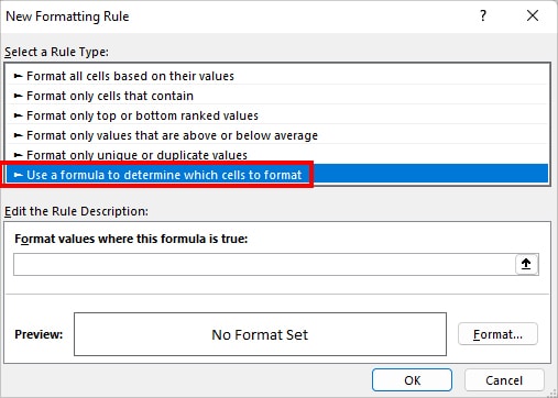
3. In New Formatting Rule window, select Use a formula to determine which cells to format option.
    
4. Now, enter the formula =ISNUMBER(SEARCH($B$2, A2)) in the Rule box. (Here, $B$2 is an empty cell that’ll function as a Search function. A2 is the first value of the data we selected above.)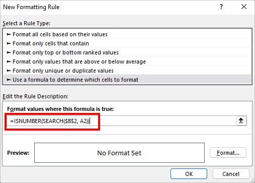
   
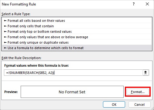
5. Click on Format.
   
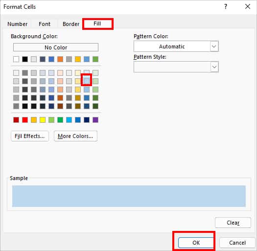
6. Head to the Fill tab on the Format Cells window. Select a Color to apply to the data and hit OK. 
   
7. Again, click OK.
8. You’ll see that the entire data is highlighted with the color. Now, on the $B$2 cell, enter a Value to search. When you do this, only the searched option will be highlighted.